Transcription
Enhancing Data Visualization TechniquesJosé Fernando Rodrigues Jr.,Agma J. M. Traina,Caetano Traina Jr.Computer Science DepartmentUniversity of Sao Paulo at Sao Carlos - BrazilAvenida do Trabalhador Saocarlense, 40013.566-590 São Carlos, SP - Brazile-mail: [junio, cesar, caetano, agma]@icmc.usp.brAbstract. The challenge in the Information Visualization (Infovis) field is two-fold: theexploration of raw data with intuitive visualization techniques and the discover of new techniquesto enhance the visualization power of well-known infovis approaches, improving the synergybetween the user and the mining tools. This work pursues the second goal, presenting the use ofinteractive automatic analysis combined with visual presentation. To demonstrate such ideas, wepresent three approaches aiming to improve multi-variate visualizations. The first approach,named Frequency Plot, combines frequencies of data occurrences with interactive filtering toidentify clusters and trends in subsets of the database. The second approach, called RelevancePlot, corresponds to assign different shades of color to visual elements according to theirrelevance to a user’s specified set of data properties. The third approach makes use of basicstatistical analysis presented in a visual format, to assist the analyst in discovering usefulinformation. The three approaches were implemented in a tool enabled with refined versions offour well-known existent visualization techniques, and the results show an improvement in theusability of visualization techniques employed.1. IntroductionThe volume of digital data generated by worldwide enterprises is increasingexponentially. Therefore, together with concerns about efficient storage and fast andeffective retrieval of information, comes the issue of getting the right information at theright time. That is, companies can gain market space by knowing more about theirclients’ preferences, usual transactions, and trends. Well-organized information is avaluable and strategic asset, providing competitive advantage on business activities.The Information Visualization (Infovis) techniques aim to take advantage of the factthat humans can understand graphical presentations much more easily and quickly,helping users to absorb the inherent behavior of the data and to recognize relationshipsamong the data elements. As a consequence, such techniques are becoming more andmore important during data exploration and analysis.Besides being voluminous, the data sets managed by the information systems arefrequently multidimensional. Thus, the process of analyzing that data is cumbersome,as this type of information is constituted by many features and properties that are hardto be apprehended by the use as a whole. Therefore, in order to bypass the intricate taskof analyzing complex data sets, we propose an alternative course for the visualizationtasks, bringing together automatic data analysis and the presentation of the results of this
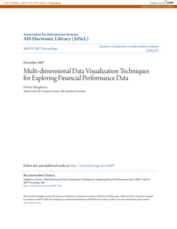
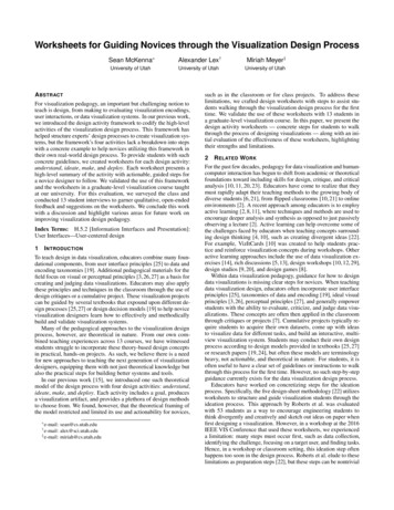
analysis in intuitive graphical formats. Following this direction we implemented threeideas in a single interactive tool.The first proposed technique, the Frequency Plot, intends to tackle two problemsderived from the increasing in the amount of data observed in most of the existingvisualization techniques. The problems are the overlapping of graphical elements, andthe excessive population of the visualization scene. The first one prevents thevisualizations to present information implicit in the “lost” elements overlapped in thescene. The second one is responsible for determining unintelligible visualizations since,due to the over-population, no tendency or evidence can be perceived.Fig. 1. - Examples of databases with too concentrated data (a),and with too spread data (b)These cases are exemplified in figure 1, using the Parallel Coordinates visualizationtechnique [1]. Figure 1(a) shows a common database where some ranges are somassively populated that only blots can be seen in the visualization scene. Therefore, thehidden elements cannot contribute for investigation. Figure 1(b) shows a hypotheticaldatabase where values in every dimension are uniformly distributed between thedimensions’ range, so the corresponding visualization becomes a meaningless rectangle.To deal with the issues pointed above, the Frequency Plot intends to increase theanalytical power of visualization techniques, allowing to weight the data to be analyzed.The analysis, based on the frequency of data occurrence, can demonstrate the areaswhere the database is most populated, while its interactive characteristic allows the userto choose the most interesting subsets where this analysis shall take place.The second technique proposed, the Relevance Plot, describes a way to analyze andto present the behavior of a data set based on a interactively defined set of properties.In this approach, the data elements are confronted with the set of properties defined bythe user in order to determine their importance according to what is more relevant to theuser. This procedure permits the verification, discovering and validation of hypothesis,providing a data insight capable of revealing the essential features of the data.The third idea is the visual presentation of basic statistical analysis along with thevisualization of a given technique. The statistical summarizations used are the average,standard deviation, median and mode.The remainder of the paper is structured as follows. Section 2 gives an overview ofthe related work and Section 3 describes the data set used in the tests presented in thiswork. Sections 4 and 5 present the Frequency Plot and Relevance Plot approaches
respectively. Section 6 shows techniques to present results of statical analysis performedover visual scenes. The tool integrating the proposed techniques is described in Section7, and the conclusions and the future works are discussed in the Section 8.2. Background and Related WorkNowadays, information visualization and visual data mining researchers face two facts:exhibition devices are physically limited, while data sets are inherently unlimited bothin size and complexity. In this scenario, the Infovis researches must improvevisualization techniques, besides finding new ones that should target large datasets. Wepropose improvements based on both interaction and automatic analysis, so theircombination might assist the user in exploring bigger data sets, more efficiently.According to [3], conventional multivariate visualization techniques do not scalewell with respect to the number of objects in the data set, resulting in displays withunacceptable cluttering. In [4], it is asserted that the maximum number of elements thatthe Parallel Coordinates technique can present is around a thousand. In fact, most of theexisting visualization techniques do not sustain interestingness when dealing with muchmore than this number, either due to space limitations inherent to current displaydevices, or due to data sets whose elements tend to be too spread over the data domain.Therefore, conventional visualization techniques often generate scenes with a reducednumber of noticeable differences.Many limitation from visualization methods can be considered inevitable becauselargely populated databases often exhibit many overlapping values, or a too spreaddistribution of data. These shortcomings lead many multi-variate visualizationtechniques to degenerate. However, some limitations have been dealt by the computerscience community in many works, as explained following.A very efficient method to bypass the limitations of overplotting visualization areasis using hierarchical clustering to generate the visualization expressing aggregationinformation. The work in [6] proposes a complete navigation system to allow the userto achieve the intended level of details in the areas of interest. That technique wasinitially developed for use with Parallel Coordinates, but implementations that comprisesmany other multivariate visualization schemes are available, as for example in the XmdvTool [3]. The drawback of this system is its complex navigation interface and the highprocessing power required by the constant re-clustering of data, according to user’sredefinition.Another approach, worth to mention, is described in [7], which uses wavelets topresent data in lower resolutions without losing the aspects of its overall behavior. Thistechnique takes advantage of the wavelets’ intrinsic property of image details reduction.Although there is a predicted data loss that might degrade the analysis capabilities, theuse of this tool can enhance the dynamic filtering activity.However, the most known and used alternative to perceive peculiarities in massivedata sets is finding ways to visually highlight subsets of data instead of the wholedatabase. The “interactive filtering principle” claims that in exploring large data sets, itis important to interactively partition the dataset into segments and focus on interestingsubsets [8]. Following this principle, many authors developed tools aiming theinteractive filtering principle, as the Magic Lenses [9] and the Dynamic Queries [10].The selective focus on the visualization is fundamental in interaction mechanisms, since
it enriches the user participation during the visualization process, allowing users toexplore the more interesting partitions in order to find more relevant information.An interesting approach in selective exploration is presented in the VisdB tool [11],which provides a complete interface to specify a query whose results will be the basisfor the visualization scene. The presentation of the data items use the relevance of itemsto determine the color of the corresponding graphical elements. The color schemedetermines the hue of the data items according to their similarity to the data itemsreturned by the query. The multi-variate technique used is pixel oriented, and theinteraction occurs based on a query form positioned alongside the visualization window.The analysis depends on the user ability to join information originating from onewindow per attribute, since each attribute is visualized in a separate scene.Another approach is the direct manipulation interaction technique applied toInformation Visualization [12], that is, techniques that improve the ability of the userto interact with a visualization scene in such a way that the reaction of the system to theuser’s activity occurs within an period short enough to the user to establish a correlationbetween their action and what happen in the scene [13]. Known as the “cause and effecttime limit” [12], this time is approximately 0.1 second, the maximum accepted timebefore action and reaction seems disjointed. Our work was oriented by this principle, sothat the tool developed satisfies this human-computer interaction requisite.3. The Breast Cancer Data SetIn the rest of this work, we present some guiding examples to illustrate the presentation.The examples use a well-known data set of breast cancer exams [2], which was built byDr. William H. Wolberg and Olvi Mangasarian from the University of Wisconsin, andis available at the University of California at Irvine Machine Learning Laboratory:(ftp://ftp.cs.wisc.edu /math-prog/cpo-dataset/machine-learn/WDBC). It comprises 457records from patients whose identities were removed. Each data item is described by 9fact attributes (dimensions), plus a numeric identifier (attribute 0), and a classifier(attribute 11) which indicates the tumor type (0 for benign and 1 for malign). The factattributes (from the 2nd to the 10th attributes) are results of analytical tests on patients'tissue samples. They might indicate the malignity degree of the breast cancer and arerespectively named ClumpThickness, UniforSize, UniforShape, MargAdhes,SingleEpithSize, BareNuclei, BlandChromatin, NormalNucleoli and Mitoses. Thesenames are meaningfull in medical domain, but do not influence the visualizationsinterpretation. Noise data was removed from the original source.4. The Frequency Plot with Interactive FilteringNow we present a new enhancement for infovis techniques, intended not only to bypassthe limits of visualization techniques previously pointed out in this text, but also toprovide a way to enhance the analytical power of every visualization techniqueembodied in an interaction mechanism. It combines interactive filtering with directmanipulation in an analytical-based presentation schema - that is, selective visualization
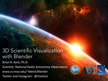
enhanced by further filtering of the selected portions of the data set is followed by anautomatic analysis step. We named this presentation technique as the Frequency Plot.Here we describe the idea in general terms, reserving an example for later detailing.By frequency, we mean how common (frequent) is a given value inside the dataset.Formally, given a set of values V {v0, v1, ., vk-1}, let q(v,V)6N be a function whichcounts how many times v 0 V appears in the set V. Also, let m(V) be a function thatreturns the statistical mode of the set V. The frequency coefficient of a value v 0 V isgiven by:(1)The function f(v,V) returns a real number between 0 and 1 that indicates howfrequently the value v is found inside the set V. In our work, this function is applied toevery value of every dimension in the range under analysis. Given a dataset C with nelements and k dimensions, its values might be interpreted as a set D with k subsets, onesubset for each dimension. That is, D {{D0},{D1},.,{Dk-1}}, having Dx n. Givena k-dimensional data item cj (cj0, cj1, ., cjk-1) belonging to set C, its correspondingk-dimensional frequency vector Fj is given by:(2)Using Equation 2, we can calculate the frequency of any k-dimensional element.Once calculated the corresponding frequencies, each object is exhibited through visualeffects as color and size modulated by its frequency. This is shown in ourimplementation in the following way. Using the Parallel Coordinates technique, thefrequencies are expressed by color, and using the Scatter Plots technique, the frequenciesare expressed by both color and size. This implementation uses a single color for eachdata item, a white background for the scene, and the high frequency values are exhibitedwith more saturated tones, in contrast with the low frequency ones, whose visualizationswere based on less visible graphical elements determined by smooth saturations, thattend to disappear in the white background.Combining the interactive filtering with this idea, our proposed visualizationtechnique is not based on the whole data set, but on selected partitions specified by theuser. These partitions are acquired by the manipulation stated by the interactive filteringprinciples, embodying AND, OR and XOR logical operators, in a way that enables theuser to select data through logical combinations of ranges in the chosen dimensions.Therefore, only the data items that satisfy the visual queries are used to perform thefrequency analysis. Hence, subsets of the database can be selected to better demonstrateparticular properties in the dataset.An illustrative example is given in figure 2. In this figure, the Frequency Plot of thecomplete dataset and the traditional range query approach are contrasted with avisualization comprising a range query with the Frequency plot. The data set underanalysis is the breast cancer database described in section 3. The analysis process isillustrated intending to clarify what is the difference between malign and benign breastcancer based on laboratory tests.In figure 2(a), the overall data distribution can be seen through the use of a globalfrequency analysis. The figure indicates the presence of more low values in most of the
dimensions. Figures 2(b) and 2(c) presents the malign and benign records respectively,using the ordinary filtering technique, where no color differentiates the data items. It isclear that these three scenes contribute little to cancer characterization, as thevisualization should do. None of them can partition nor analyze data simultaneously and,consequently, they are incapable of supporting a consistent parsing of the problem.In contrast, figures 2(d) and 2(e) better demonstrate the characteristics relative to thelaboratory tests and cancer nature. In these figures, the attribute 1, class, is used todetermine frequency, considering value 0 (benign) in figures 2(d) and value 1 (malign)in figure 2(e). By highlighting the most populated areas of the selections, malign andbenign cancer turns out to be identified more easily by searching for patterns alike thosethat are made explicit by the Frequency Plot. Therefore, the analyst is enabled toconclude what results he/she needs to search for in order to make the characterizationof the cancer nature more precise. The data distribution is visually noticeable and canbe separately appreciated due to the interactive filtering.Fig. 2 - Parallel Coordinates with Frequency Plot. (a) The frequency analysis of the whole dataset; (b) the traditional visualization of the malign class 1; (c) the benign class 0 visualization.(d) Frequency Plot of (b); (e) the correspondent Frequency Plot of (c)
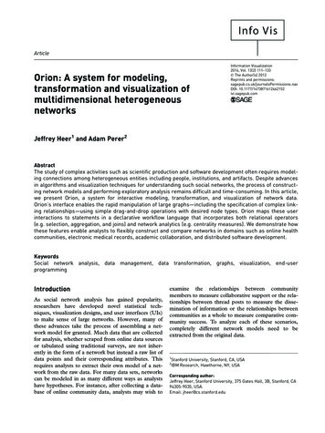
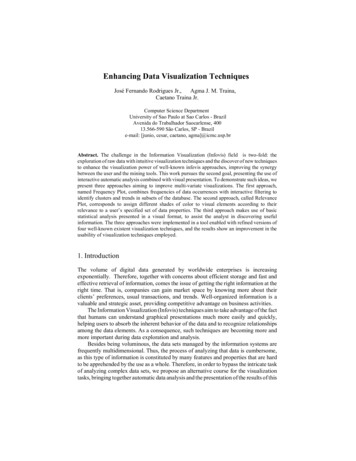
Figure 3 shows the same visualizations as were presented in figure 2, but in a ScatterPlots Matrix enhanced by the Frequency Plot analysis. The Scatter Plots visualizationcorroborates what has been already seen in the Parallel Coordinates scenes and it furtherclarifies the fact that the “BlandChromation” and the “SingleEpithSize” attributes are theless discriminative in cancer nature classification.The data presentation with frequency plot is a powerful tool because it candetermine more easely the subset of interest for the analysis. Also, it points that clusteridentification is not limited to the whole data set, nor to predefined manipulated dataFig. 3 - (a) The Scatter Plot Matrix with Frequency Plot showing the benign cancer autopsies.Note the zoom of the “BlandChromation” attribute. (b) Correspondente visualization of themalign cancer autopsies and the zoom of the “SingleEpithSize” attribute
records. Instead, it might occur guided by a single value. One might choose a densepopulated area belonging to one of the dimensions and questions the reason of thatbehavior. The frequency plot technique will present the most frequent values of the otherdimensions that are correlated to the region of interest; correlation goes straight alongwith partial cluster identification.5. The Relevance PlotThe second technique described in this work is based on the concept of data relevance,showing the information according to the user’s needs or sensibility. Therefore, weintend to reduce the amount of information presented by drawing data items using visualgraphic patterns in accordance to their relevance to the analysis. That is, if the data hasa strong impact on the information under analysis, their visualization shall stress thisfact, and the opposite must happen to data that is not relevant to the user. To this intent,the Relevance Plot benefits from computer graphic techniques applied to depictautomatic data analysis through color, size, position and selective brightness.The proposed interaction does not depend on a query stated on a Structured QueryLanguage (SQL) command, thus it is not based on a set of range values, but rather, it isbased on a set of values considered interesting by the user. These values are used todetermine how relevant is each data item. Once the relevant characteristics are set,automatic analysis proceeds through calculation of data relevance relative to what waschosen by the user to be more interesting.The mechanism is exemplified in Figure 4. It requires the analyst to choose values,or Relevance Points, from the dimensions being visualized. Hence, given a set of dataitems C with n elements and k dimensions, and assuming that these values werepreviously normalized so that each dimension ranges from 0.0 to 1.0, the followingdefinitions hold:Definition 1: the Relevance Point (RP) of the i-th dimension, or RPi, is thechosen value belonging to the i-th dimension domain that must be considered todetermine the data relevance in that dimension.For illustration purposes, let us first consider only one RP per dimension. Once theRelevance Points are set for every dimension, the data items belonging to the databasemust be analyzed considering their similarity to these points of relevance. That is, foreach dimension with a chosen RP, all the values of every tuple is computed consideringtheir Euclidean distance to the respective relevance value.Definition 2: for the j-th k-dimensional data record cj (cj0, cj 1 ,., cj k-1), thedistance of its i-th attribute to the i-th RP, or Dji(cji, RPi), is given by:(3)We use the Euclidean distance due to its simplicity, but other distances, such as anymember of the Minkowski family, can also be employed. For each dimension of thek-dimensional database, a maximum acceptance distance can be defined. Thesethresholds are called Max Relevance Distances, or MRDs, and are used in the relevanceanalysis.
Fig. 4 - The Relevance Plot schema is demonstrated here through the calculus of therelevance for a 4-dimensional sample record visualized in the Parallel CoordinatestechniqueDefinition 3: the Max Relevance Distance of the i-th dimension, or MRDi, is themaximum distance Dji(cji, RPi) that a data attribute can assume, before itsrelevance assume negative values during relevance analysis. The MRDs takevalues within the range [0.0, 1.0].Based on the MRDs and on the calculated distances Dji(cji, RPi), a value namedAttribute Relevance (AR) is computed for each attribute of the k-dimensional data items.Thus, a total of k ARs are computed for each of the n k-dimensional data items in thedatabase.Definition 4: the value determining the contribution of the i-th attribute of thej-th data item, cji in the relevance analysis is called the Attribute Relevance, andis given by:(4)Equation 4 states that: For distances D(c,RP) smaller or equal the MRD, the equation has been settled toassign values ranging from 1 (where the distances D(c,RP) are null) to 0 (fordistances equal the MRD);
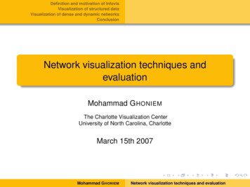
For distances D(c,RP) bigger than the MRD, the equation linearly assigns valuesranging from 0 to -1; In dimensions without a chosen RP, the AR assumes a value 0 and does not affectanalysis.Finally, after processing every value of the dataset, each of the k-dimensional itemwill have a value computed, that is called Data Relevance (DR) and stands for therelevance of a complete information element (an tuple with k attributes).Definition 5: the Data Relevance (DR) is the computed value that describes howrelevant a determined data item is, based on the Attribute Relevancies. So, fora given data item, the DR is the average of its correspondent AttributeRelevancies. For the j-th k-dimensional element of a data set, the DRj is givenby:(5)where #R is the number of Relevance Points that were defined for the analysis.The Data Relevance value directly denotes the importance of its corresponding dataelement, according to the user defined Relevance Points. To visually explicit this fact,we use the DRs to determine the color and size of each graphic elements. Hence, a lowerDR stands for weaker saturations and smaller sizes, while higher ones stand for morestressed saturations and bigger sizes. In our implementation we benefit from the factthat only the saturation component is necessary to denote relevance, leaving the othervisual attributes (colors, hue and size) available to depict other associated information.In this sense, we projected a way to denote, along with the relevance analysis, theaforementioned frequency analysis.That is, while the saturation of color and the size of the graphical elements denoterelevance, the hue component of color presents the frequency analysis of the data set.More precisely, the highest frequencies are presented in red (hot) tones, and the lowestfrequencies in blue (cold) tones, varying linearly passing through magenta.Figure 5 presents the usage of the Relevance Plot technique over the ParallelCoordinates technique using the breast cancer dataset. In the three scenes we havedefined 9 Relevance Points for dimensions 2 to 10. For illustration purposes in Figure5(a), the points are set to the smallest values of each dimension, in Figure 5(b) they areset to the maximum values of each dimension, and in Figure 5(c) they are to the middlepoints. However, each dimension can have its RP defined at the user’s discretion.In figure 5(a) the choice of the Relevance Points and their correspondentvisualization leads to conclude that the lowest values of the dimensions’ domainsindicate class 0 (benign cancer) records. It also warns that this is not a final conclusionsince the visualization reveals some records, in lower concentration, which are classifiedas 1 (malign cancer). It can be said that false negative cancer analysis can occurconsidering a clinical approach based on this condition.In figure 5(b) the opposite can be observed, as the highest values indicate therecords of class 1. It can be seen that false positive cancer analysis can also occur, butthey are less common that the false negative cases, since just a thin shadow of pixelsheads to class 0 in the 11th (right most) dimension.
Finally, in figure 5(c) the Relevance Points were set to middle points in order tomake an intermediate analysis. In this visualization, one can conclude that this kind oflaboratory analysis is quite categorical, since just one record is positioned in the middleof the space determined by the dimensions’ domains. But, in such cases, it is wise toclassify the analysis as a malign cancer or, otherwise, to proceed with more exams.Fig 5 - The Relevance Plot over a Parallel Coordinates scene. In (a) all therelevance points are set to the smallest values of their dimensions. In (b) theyare set to the maximum values and in (c) middle points are set
6. Basic Statistics PresentationThe statistical analysis has been successfully applied in practically every research fieldand its use in Infovis naturally improves data summarization. So, defending our idea thatinformation visualization techniques must be improved by automatic analysis, this paperdescribe how our visualization tool makes use of basic statistics to complement therevealing power of traditional visualization mechanisms.The statistical properties we used take advantage of are the average, standarddeviation, median and mode values, and the method for visualizing them isstraightforward. The raw visualization scene is rendered, and the statisticalsummarizations are used to draw an extra graphical element over the image. The extragraphic elements are the summarizations which are exhibited with a different color forvisual emphasis.The four statistical summarizations are available in each of the four visualizationtechniques implemented in the GBDIView tool, which will be presented in the nextsection. As an example, figure 6 presents the breast cancer dataset drawn using the StarCoordinates technique together with a polygon over the scene indicating the medianvalues of the malign cancer exams (figure 6.a) and of the benign cancer exams (figure6.b). Also in figure 6, we can see the same data set drawn using the Parallel Coordinatestechnique together with a polyline indicating the average values of the malign cancerexams (figure 6.c) and of the benign cancer exams (figure 6.d). The possibilities of thesevisualization schemes are very promising, being more powerful than their respectiveraw visualizations using the Star Coordinates and Parallel Coordinates techniques. In ashort analysis, the presented statistical visualization stress the conclusions addressed bythe examples shown in sections 4 and 5.Fig. 6 - In (a) the median of the malign cancer exams presented over the Star Coordinates; in (b)the median of the benign exams. In (c) the average line of the malign cancer exams over theParallel Coordinates and in (d) the average of the benign exams
7. The GBDIView ToolIn order to experiment our ideas, we have implemented a tool whose snapshot ispresented in figure 7, that fully encompass the theory presented in this paper. TheGBDIView tool consists of 4 well-known visualization techniques enhanced by theproposed approaches we have developed. The tool is built in C , and was designedfollowing the software reuse paradigm, therefore, being idealized as a set ofvisualization methods implemented as software components that can be totally tailoredto any software that uses Infovis concepts.The techniques included in the tool are the Parallel Coordinates, the Scatter PlotsMatrix [5], the Star Coordinates [14] and the Table Lens [15]. The four visual schemesare integrated by the Link & Brush [16] technique and every one is also enabled with theFrequency Plot, with the Relevance Plot and with the statistical data analysis (average,standard deviation, median and mode values), what can be presented graphically overthe rendered scenes.A fully functional version of the tool, along with its user's guide and some sampledatasets can be obtained at http://gbdi.icmc.usp.br/ junio/GBDIViewTool.htm.8. Conclusions and Future WorkWe believe that both the Frequency Plot and the Relevance Plot techniques can stronglycontribute to improve the effectiveness of databases exploration, specially the relevancevisualization, which is a way to focus on interesting parts of a data set without losing theoverall sight. We also argue that this contribution is applicable to other multi-variateFig. 7 - The GBDIView tool presenting a Table Lens visualization with Relevance Plot
visualization techniques beyond the Parallel Coordinates, the Scatter Plots, the StarCoordinates and the Table Lens, some of which are already implemented in theGBDIView tool.It is important to observe that the contributions of this work are not limited to thetechn
Nowadays, information visualization and visu al data mining researchers face two facts: exhibition devices are physically limited, while data sets are inherently unlimited both . A very efficient method to bypass the limitations of overplotting visualization areas is using hierarchical clustering to generate the visualization expressing .