WIXLIB

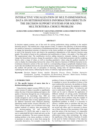
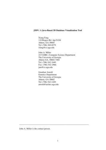
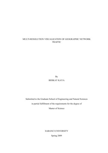
Marghescu, Multidimensional Visualization Techniques for Financial Performance DataPermutation 5060.8440.9721.101.23-18.63-38.50ROTAThe permutation matrix is a special type of bar graph described by Bertin (1983). In a permutation matrix, each datadimension is represented by a bar graph in which the heights of the bars represent the data values. The horizontal axes of allbar graphs have the same information (e.g., the time or ordering of the data table). The below average data values arecoloured black, and the above average data values are coloured white. A green dashed line plotted over the data representsthe average value of each dimension. Implementations of permutation matrixes allow the interactive changing of the order ofthe records for observing interesting patterns.Figure 2 displays a permutation matrix created with Visulab (Hinterberger and Schmid 1993). On the horizontalaxes the companies are arranged in descending order of ROTA. The companies of interest are highlighted. This graphfacilitates the detection of relationships between ratios and the comparison of companies. It also reveals anomalies in 1.4.1.1.8.6.5.1.2.3.1.8.C DBFigure 2 Permutation matrix created with VisulabASurvey plotThe survey plot is a variation of the permutation matrix. The values of each data dimension are represented ashorizontal bars. The width of the bars is proportional to the data values. The bars are centred and there are no spacesseparating the bars. One can use colours to distinguish between different classes in the data (if a class variable is present).Figure 3 displays a survey plot, in which the data are sorted according to ROTA. This facilitates the detection ofrelationships between ROTA and other ratios, for example OM, ROE and IC.Companies from different regions are displayed with different colours. The graph shows that the Japanesecompanies are not among the most profitable ones, while the American and European companies display the highestprofitability. The technique facilitates the detection of outliers and comparison between two or more companies.Scatter-plot matrixA scatter plot is used to plot two dimensional data so that the horizontal axis shows the values of one variable andthe vertical axis shows the values of another variable. The scatter-plot matrix is useful for looking at all possible pairs ofvariables in the dataset.Figure 4 displays a scatter plot matrix for three financial ratios (OM, ROE and RT). The plots reveal relationshipsbetween ROE and OM. The visualization also reveals outliers, and facilitates the comparison of companies.4

Marghescu, Multidimensional Visualization Techniques for Financial Performance DataC - Buckeye T. 1998D – Donohue 1998B – Reno deMedici 1998A - Reno deMedici 1997Figure 3 Survey plot created with Orange (Demsar 2004)ROE60.8436.0111.17-13.67-38.50Legend:A – Reno de Medici 1997B – Reno de Medici 1998C – Buckeye Technologies 1998D – Donohue 62-6.363.30-16.02RT17.5213.389.245.100.97ROEFigure 4 Scatter-plot matrix created with VisulabParallel coordinatesIntroduced by Inselberg (1985), parallel coordinates represent multidimensional data using lines. The datadimensions are represented as parallel axes (coordinates). The maximum and minimum values of each dimension are scaledto the upper and lower points on a vertical axis. An n-dimensional data point is displayed as a polyline that crosses each axisat a position proportional to its value for that dimension.Figure 5 represents the financial ratios as parallel axes and each company as a polyline that crosses each axis at apoint proportional to the value of the ratio for the corresponding company. The companies of interest are highlighted usingdifferent colours.5

Marghescu, Multidimensional Visualization Techniques for Financial Performance ure 5 Parallel coordinates created with VisulabThe display facilitates detection and characterization of outliers. One can compare the financial performance ofdifferent companies. The relationships between two or more variables can be detected if the correlated variables are arrangedconsecutively (for example, ROE and ROTA).TreemapsThe treemaps (Johnson and Shneiderman 1991) are hierarchical visualizations of multidimensional data. Datadimensions are mapped to the size, position, colour, and label of nested rectangles.Figure 6 displays the dataset using the treemaps technique. The figure was created with Treemap 4.1 (2004). Eachcompany is represented by a rectangle. The size of the rectangle indicates the value of RT. The colour of the rectangleindicates the value of the ROTA ratio as follows: light green indicates high values of ROTA; light red indicates small valuesof ROTA; dark red and dark green shows values of ROTA close to 14 (see the “colour binning” panel in the visualizationbelow). In this visualization, the dataset is organised into categories such as year and region.Figure 6 Treemap created with Treemap 4.1This treemap representation shows where the most profitable companies in terms of ROTA are located, and how thecompanies of interest have evolved over time. In addition, one can identify common features or patterns in the industry, for6

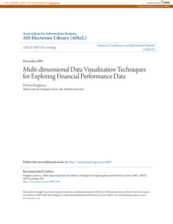
Marghescu, Multidimensional Visualization Techniques for Financial Performance Dataexample, that Japanese companies have the lowest values of the efficiency ratio. One can also compare the financialperformance of different companies.Principal component analysis (PCA)PCA is a dimensionality-reducing technique employing linear transformation of data (Sharma 1995). The projectionof high-dimensional data onto a lower-dimensional space tries to preserve the variance of the original data as well aspossible. The PCA technique creates new variables (called principal components), which are linear composites of the originalvariables and are uncorrelated amongst themselves. The maximum number of new variables that can be formed is equal tothe number of original variables. The PCA output is judged in terms of how well the new variables represent the informationcontained in data, or, geometrically, how well the new dimensions can capture the original configuration of the data.Figure 7 shows PCA plot that was constructed from the standardized dataset. The red dot shows the observationclosest to the centre of the dataset. The companies of interest are marked with a yellow star and labelled on the graph.One can interpret the principal components by inspecting the loadings of each original variable to the PCs. Thehigher the loading of a variable, the more influence it has in forming the PC score and vice versa. In our case, the first PC(horizontal axis) is highly correlated with the profitability ratios and the IC ratio. Therefore, companies placed towards theright of the horizontal axis, have high values in profitability and IC. The second PC (vertical axis) is highly correlated withQR and EC. Companies located on the upper part of the graph have a high liquidity and high solvency. The amount ofvariation explained by the two PCs is 40.926% 19.455% 60.38% of the total variance. While this amount of varianceaccounts for the variation of six of the ratios, it does not consider the variation of efficiency (RT) among the companies.7Second Principal Component- highly correlated with Quick Ratio and Equity to Capital65Legend:- Companies that havethe highest values for ROTA- The company closestto the centre of the dataset43III21Reno de medici 19970Donohue 1998-1Buckeye Technologies 1998Reno de medici 1998-2-3-8III-6IV-4-2024First Principal Copmonent- highly correlated with the profitability ratios and the Interest Coverage ratio6Figure 7 Data projected on the first two PCs created with the Statistics Toolbox (The MathWorks 2002). In area I:medium-high liquidity, low-medium profitability; II: medium-high liquidity, solvency and profitability; III: lowmedium liquidity, solvency and profitability; IV: low-medium liquidity, medium-high profitabilityIn addition to its usefulness as a data reduction method, PCA is also useful in finding numerous patterns in data(Figure 7). The graph shows the high profitability of Buckeye Technologies 1998 and Donohue 1998, and the increase inprofitability for Reno and Medici in 1998. The high correlation of the first PC with all profitability ratios and with the ICratio indicates that there also exists a relationship between the profitability ratios and IC. Similarly, the high correlation of thesecond PC with EC and QR indicates that EC and QR are also correlated.7

Marghescu, Multidimensional Visualization Techniques for Financial Performance DataBy splitting the visual representation in four areas by two orthogonal lines that intersect in the centre of the dataset,one can divide the dataset into four groups of similar observations as shown and described in Figure 7. Based on the meaningof the first two PCs, one can conclude that in area I there are companies with medium-high liquidity and low-mediumprofitability; in area II, companies with medium-high liquidity, solvency and profitability; in area III, companies with lowmedium liquidity, solvency and profitability; and in area IV, companies with low-medium liquidity but medium-highprofitability. Based on this evaluation, one can compare the financial performance of the companies of interest.Sammon’s mappingSammon’s mapping is a nonlinear projection of the multidimensional data down to two dimensions so that thedistances between data points are preserved (Kohonen 2001). It belongs to multidimensional scaling techniques.Figure 8 illustrates our financial dataset using Sammon’s mapping. The data values were normalized using thediscrete histogram equalization method. The normalization method works in two steps: first, the data values of each variableare replaced by the order index, and then these values are normalized to be in the range [0, 1], by applying a lineartransformation. Companies from different regions are displayed using different colours. The companies of interest are markedwith yellow stars and labelled on the graph.1.5EuropeN EuropeUSACanadaJapan10.5Reno de Medici 19970Buckeye Technologies 1998Reno de Medici 1998Donohue 1998-0.5-1-1.5-1.5-1-0.500.511.5Figure 8 Sammon’s mapping created with SOM Toolbox 2.0 (2005)The technique is useful in visualizing class distributions, especially the degree of their overlap. One can see thatcompanies from Canada and USA overlap and map to the same area of the graph, whereas Japan, Europe and NorthernEurope form three separate groups. However, the degree of overlapping between all these classes is quite high; especiallyEurope and Northern Europe do not separate well from the other groups. The differences and similarities between thecompanies are easy to distinguish, but not easy to interpret.Self-Organizing Maps (SOM)The SOM technique, developed by Kohonen (2001) is a special type of neural network based on unsupervisedlearning. The SOM algorithm is similar to the K-Means clustering algorithm, but the output of a SOM is topological andneighbouring clusters are similar. As a projection technique of multidimensional data onto a two-dimensional grid, the SOMmethod is similar to multidimensional scaling techniques, such as Sammon’s mapping. The grid consists of units that haveassigned reference vectors with the same dimensionality as the original data. After learning is complete, the reference vectorsare updated such that they resemble most of the data items, as much as possible. Each data item is then mapped to the unitwhere the highest similarity between the reference vector and the data item is calculated. Multiple data items mapped ontothe same unit are similar and form a cluster.8

Marghescu, Multidimensional Visualization Techniques for Financial Performance DataWe have used the SOM technique on normalized data obtained byapplying the d iscrete histogram equalizationmethod. There are many ways to represent the SOM output. One way to represent the data is to use the scatter plot technique(usually with jittering), in which the horizontal and vertical axes are produced by the Kohonen network (i.e., the map size, inour case 6x5 units).Figure 9 is a scatter plot of the dataset based on the SOM coordinates. Companies from different regions arehighlighted using different colours. The technique of jittering was used in order to change with a small value the position ofeach company; otherwise the companies mapped to the same unit would have overlapped. Figure 9 shows many clusters inthe data (if more companies are mapped to the same map unit, they may be interpreted as forming a cluster). One can alsoobserve some isolated companies. However, the interpretability of this map is not easy. One can distinguish among thecompanies belonging to the same region, or identify the placement of these companies on the map but cannot interpret theseclasses or the clusters formed.43.5Reno de medici 19973EuropeN EuropeUSA2.5CanadaJapanMap units21.5Reno de medici 199810.50Donohue 1998Buckeye Technologies 1998-0.5-10123456Figure 9 Self-Organizing Map – scatter plot view created with SOM Toolbox 2.0Ultsch and Siemon (1989) developed the U-matrix graphic display to illustrate the clustering of the referencevectors, by representing graphically the distances between map units. In this visual representation, each map unit is typicallyrepresented by a hexagon. The line or border between two neighbouring map-units (hexagons) has a distinguishable colourthat signifies the distance between the two corresponding reference vectors. Dark green signifies for large distances, and lightgreen signifies similarities between the vectors, as indicated by the colour bar (Figure 10-Left).AA1B234BC, DC,DFigure 10 Left: Self-Organizing Map - U-matrix view created with Nenet 1.1 (1999); Right: Clustering of SOM viewcreated with SOM Toolbox 2.0By looking at the borders’ colours in Figure 10-Left, one can distinguish the main clusters that exist in the data. Aclustering algorithm (e.g., K-means) can be used to automatically partition the map into similar clusters (Figure 10-Right),creating the clustering of SOM view. The dataset appears to contain four main clusters. Based on Figure 9 and Figure 10, onecan compare the companies of interest with respect to their membership in the identified clusters. Moreover, one can see the9

Marghescu, Multidimensional Visualization Techniques for Financial Performance Datacomposition of each cluster with respect to the variable Region (e.g., Cluster 4 contains mostly American, Northern Europeanand European companies).It is also possible to visualize each data dimension using feature planes. These represent graphically the levels of thevariables in each map unit. The colour red signifies high values of the variables, and blue and black correspond to low valuesof the variables (as indicated by the colour bars, Figure C,D5.28dC,D2.4d0.893B33.4dC,D0.744dQRFigure 11 Feature planes created with SOM Toolbox 2.0The feature planes facilitate the comparison of the companies of interest. The feature planes also help to identify therelationships between variables (e.g., OM is correlated with ROE; EC is correlated with QR).By examining the features planes in parallel with the clustering of the SOM, one obtains the description of the fourclusters identified previously as follows. Cluster 1 shows very low profitability, liquidity, solvency and efficiency. It containsthe companies with the poorest financial performance. Reno de Medici 1997 is situated in this cluster (A). Cluster 2 showsmedium profitability, solvency, and liquidity, but low efficiency. Reno de Medici 1998 belongs to this cluster (B). Cluster 3shows good profitability, liquidity and solvency. Efficiency is medium to low. Cluster 4 shows very high profitability,solvency, liquidity and efficiency. It contains the companies with the best financial performance, among which BuckeyeTechnologies 1998 and Donohue 1998 (C and D) are situated.Comparison of visualization techniquesIn the previous section, we illustrated the use of multidimensional data visualization techniques for exploringfinancial performance data. All visualization techniques used are capable of providing an overview of the dataset underanalysis, and different techniques uncover different patterns in the data. We highlighted the capabilities of each technique foranswering the business questions and data mining tasks related to the financial benchmarking problem. In this section, wecompare the techniques with respect to three criteria: 1) their capabilities to answer the questions and data mining tasksformulated for the financial benchmarking problem; 2) their capabilities to show data items or data models; and 3) the type ofdata used as input for the visualization technique (i.e., original data or normalized data).First, we provide in Table 2 a subjective comparison of the techniques with respect to their capabilities for solvingthe data mining tasks related to financial benchmarking. The assessment concerns only this business problem and theassociated dataset. We do not intend to generalize the results to other datasets, because for a different dataset (with differenttypes of data, number of variables, number of observations, underlying structure) the results of the evaluation could bedifferent. Table 2 can be used as a means to map the data mining tasks to different visualization techniques for this dataset.This table can, therefore, be used in the process of selection of visualization techniques suitable for representing andexploring the data in the financial benchmarking problem.Table 2 shows that there are data mining tasks for which more than one visualization technique can be used. On theother hand, one data mining task may be addressed using different visualization techniques but with a different outcome (e.g.,clustering solutions produced by the SOM and PCA). Almost all visualization techniques can facilitate the comparisonamong companies. M

Keywords: multidimensional data visualization techniques ; financial performance ; financial data visualization Introduction Many novel visualization techniques have been developed i n the field s of information visualizat ion (Card et al. 1999) and visual data mining (Keim 2002) . However, t he research literature concerning the use of visual .