WIXLIB

10CONTENTSPrequisitesIt’s assumed that you have some experience with the R language and that you have already installed R andRStudio. If not, here are some resources for getting started: A (very) short introduction to RDataCamp - Introduction to R with Jonathon CornelissenQuick-RGetting up to speed with RSetupIn order to create the graphs in this guide, you’ll need to install some optional R packages. To install all ofthe necessary packages, run the following code in the RStudio console window.pkgs - c("ggplot2", "dplyr", "tidyr","mosaicData", "carData","VIM", "scales", "treemapify","gapminder", "ggmap", "choroplethr","choroplethrMaps", "CGPfunctions","ggcorrplot", "visreg","gcookbook", "forcats","survival", "survminer","ggalluvial", "ggridges","GGally", "superheat","waterfalls", "factoextra","networkD3", "ggthemes","hrbrthemes", tively, you can install a given package the first time it is needed.For example, if you executelibrary(gapminder)and get the messageError in library(gapminder) : there is no package called ‘gapminder’you know that the package has never been installed. Simply executeinstall.packages("gapminder")once andlibrary(gapminder)will work from that point on.

Chapter 1Data PreparationBefore you can visualize your data, you have to get it into R. This involves importing the data from anexternal source and massaging it into a useful format.1.1Importing dataR can import data from almost any source, including text files, excel spreadsheets, statistical packages, anddatabase management systems. We’ll illustrate these techniques using the Salaries dataset, containing the 9month academic salaries of college professors at a single institution in 2008-2009.1.1.1Text filesThe readr package provides functions for importing delimited text files into R data frames.library(readr)# import data from a comma delimited fileSalaries - read csv("salaries.csv")# import data from a tab delimited fileSalaries - read tsv("salaries.txt")These function assume that the first line of data contains the variable names, values are separated by commasor tabs respectively, and that missing data are represented by blanks. For example, the first few lines of thecomma delimited file looks like 00Options allow you to alter these assumptions. See the documentation for more details.11

121.1.2CHAPTER 1. DATA PREPARATIONExcel spreadsheetsThe readxl package can import data from Excel workbooks. Both xls and xlsx formats are supported.library(readxl)# import data from an Excel workbookSalaries - read excel("salaries.xlsx", sheet 1)Since workbooks can have more than one worksheet, you can specify the one you want with the sheet option.The default is sheet 1.1.1.3Statistical packagesThe haven package provides functions for importing data from a variety of statistical packages.library(haven)# import data from StataSalaries - read dta("salaries.dta")# import data from SPSSSalaries - read sav("salaries.sav")# import data from SASSalaries - read sas("salaries.sas7bdat")1.1.4DatabasesImporting data from a database requires additional steps and is beyond the scope of this book. Depending onthe database containing the data, the following packages can help: RODBC, RMySQL, ROracle, RPostgreSQL,RSQLite, and RMongo. In the newest versions of RStudio, you can use the Connections pane to quickly accessthe data stored in database management systems.1.2Cleaning dataThe processes of cleaning your data can be the most time-consuming part of any data analysis. The mostimportant steps are considered below. While there are many approaches, those using the dplyr and tidyrpackages are some of the quickest and easiest to idyrtidyrselectfiltermutatesummarizegroup bygatherspreadselect variables/columnsselect observations/rowstransform or recode variablessummarize dataidentify subgroups for further processingconvert wide format dataset to long formatconvert long format dataset to wide format

1.2. CLEANING DATA13Examples in this section will use the starwars dataset from the dplyr package. The dataset providesdescriptions of 87 characters from the Starwars universe on 13 variables. (I actually prefer StarTrek, but wework with what we have.)1.2.1Selecting variablesThe select function allows you to limit your dataset to specified variables (columns).library(dplyr)# keep the variables name, height, and gendernewdata - select(starwars, name, height, gender)# keep the variables name and all variables# between mass and species inclusivenewdata - select(starwars, name, mass:species)# keep all variables except birth year and gendernewdata - select(starwars, -birth year, -gender)1.2.2Selecting observationsThe filter function allows you to limit your dataset to observations (rows) meeting a specific criteria.Multiple criteria can be combined with the & (AND) and (OR) symbols.library(dplyr)# select femalesnewdata - filter(starwars,gender "female")# select females that are from Alderaannewdata - select(starwars,gender "female" &homeworld "Alderaan")# select individuals that are from# Alderaan, Coruscant, or Endornewdata - select(starwars,homeworld "Alderaan" homeworld "Coruscant" homeworld "Endor")# this can be written more succinctly asnewdata - select(starwars,homeworld %in% c("Alderaan", "Coruscant", "Endor"))1.2.3Creating/Recoding variablesThe mutate function allows you to create new variables or transform existing ones.

14CHAPTER 1. DATA PREPARATIONlibrary(dplyr)# convert height in centimeters to inches,# and mass in kilograms to poundsnewdata - mutate(starwars,height height * 0.394,mass mass* 2.205)The ifelse function (part of base R) can be used for recoding data. The format is ifelse(test, returnif TRUE, return if FALSE).library(dplyr)# if height is greater than 180# then heightcat "tall",# otherwise heightcat "short"newdata - mutate(starwars,heightcat ifelse(height 180,"tall","short")# convert any eye color that is not# black, blue or brown, to othernewdata - mutate(starwars,eye color ifelse(eye color %in% c("black", "blue", "brown"),eye color,"other")# set heights greater than 200 or# less than 75 to missingnewdata - mutate(starwars,height ifelse(height 75 height 200,NA,height)1.2.4Summarizing dataThe summarize function can be used to reduce multiple values down to a single value (such as a mean). Itis often used in conjunction with the by group function, to calculate statistics by group. In the code below,the na.rm TRUE option is used to drop missing values before calculating the means.library(dplyr)# calculate mean height and massnewdata - summarize(starwars,mean ht mean(height, na.rm TRUE),mean mass mean(mass, na.rm TRUE))newdata## # A tibble: 1 x 2##mean ht mean mass

1.2. CLEANING DATA#### 1 dbl 174.15 dbl 97.3# calculate mean height and weight by gendernewdata - group by(starwars, gender)newdata - summarize(newdata,mean ht mean(height, na.rm TRUE),mean wt mean(mass, na.rm TRUE))newdata################# A tibble: 5 x 3gendermean ht mean wt chr dbl dbl 1 female165.54.02 hermaphrodite175. 1358.3 male179.81.04 none200.140.5 NA 120.46.31.2.5Using pipesPackages like dplyr and tidyr allow you to write your code in a compact format using the pipe % % operator.Here is an example.library(dplyr)# calculate the mean height for women by speciesnewdata - filter(starwars,gender "female")newdata - group by(species)newdata - summarize(newdata,mean ht mean(height, na.rm TRUE))# this can be written asnewdata - starwars % %filter(gender "female") % %group by(species) % %summarize(mean ht mean(height, na.rm TRUE))The % % operator passes the result on the left to the first parameter of the function on the right.1.2.6Reshaping dataSome graphs require the data to be in wide format, while some graphs require the data to be in long format.You can convert a wide dataset to a long dataset usinglibrary(tidyr)long data - gather(wide data,key "variable",value "value",sex:income)

16CHAPTER 1. DATA PREPARATIONTable 1.2: Wide 518income550007500090000Table 1.3: Long rsely, you can convert a long dataset to a wide dataset usinglibrary(tidyr)wide data - spread(long data, variable, value)1.2.7Missing dataReal data are likely to contain missing values. There are three basic approaches to dealing with missingdata: feature selection, listwise deletion, and imputation. Let’s see how each applies to the msleep datasetfrom the ggplot2 package. The msleep dataset describes the sleep habits of mammals and contains missingvalues on several variables.1.2.7.1Feature selectionIn feature selection, you delete variables (columns) that contain too many missing values.data(msleep, package "ggplot2")# what is the proportion of missing data for each variable?pctmiss - colSums(is.na(msleep))/nrow(msleep)round(pctmiss, 2)############name0.00sleep total0.00bodywt0.00genus0.00sleep rem0.27vore0.08sleep cycle0.61order conservation0.000.35awakebrainwt0.000.33Sixty-one percent of the sleep cycle values are missing. You may decide to drop it.

1.2. CLEANING DATA1.2.7.217Listwise deletionListwise deletion involves deleting observations (rows) that contain missing values on any of the variables ofinterest.# Create a dataset containing genus, vore, and conservation.# Delete any rows containing missing data.newdata - select(msleep, genus, vore, conservation)newdata - na.omit(newdata)1.2.7.3ImputationImputation involves replacing missing values with “reasonable” guesses about what the values would havebeen if they had not been missing. There are several approaches, as detailed in such packages as VIM, mice,Amelia and missForest. Here we will use the kNN function from the VIM package to replace missing valueswith imputed values.# Impute missing values using the 5 nearest neighborslibrary(VIM)newdata - kNN(msleep, k 5)Basically, for each case with a missing value, the k most similar cases not having a missing value are selected.If the missing value is numeric, the mean of those k cases is used as the imputed value. If the missing valueis categorical, the most frequent value from the k cases is used. The process iterates over cases and variablesuntil the results converge (become stable). This is a bit of an oversimplification - see Imputation with RPackage VIM for the actual details.Important caveate: Missing values can bias the results of studies (sometimes severely). If youhave a significant amount of missing data, it is probably a good idea to consult a statistician ordata scientist before deleting cases or imputing missing values.

18CHAPTER 1. DATA PREPARATION

Chapter 2Introduction to ggplot2This section provides an brief overview of how the ggplot2 package works. If you are simply seeking code tomake a specific type of graph, feel free to skip this section. However, the material can help you understandhow the pieces fit together.2.1A worked exampleThe functions in the ggplot2 package build up a graph in layers. We’ll build a a complex graph by startingwith a simple graph and adding additional elements, one at a time.The example uses data from the 1985 Current Population Survey to explore the relationship between wages(wage) and experience (expr).# load datadata(CPS85 , package "mosaicData")In building a ggplot2 graph, only the first two functions described below are required. The other functionsare optional and can appear in any order.2.1.1ggplotThe first function in building a graph is the ggplot function. It specifies the data frame containing the data to be plotted the mapping of the variables to visual properties of the graph. The mappings are placed within theaes function (where aes stands for aesthetics).# specify dataset and mappinglibrary(ggplot2)ggplot(data CPS85,mapping aes(x exper, y wage))Why is the graph empty? We specified that the exper variable should be mapped to the x-axis and that thewage should be mapped to the y-axis, but we haven’t yet specified what we wanted placed on the graph.19

20CHAPTER 2. INTRODUCTION TO GGPLOT240wage302010002040experFigure 2.1: Map variables

2.1. A WORKED EXAMPLE2.1.221geomsGeoms are the geometric objects (points, lines, bars, etc.) that can be placed on a graph. They are addedusing functions that start with geom . In this example, we’ll add points using the geom point function,creating a scatterplot.In ggplot2 graphs, functions are chained together using the sign to build a final plot.# add pointsggplot(data CPS85,mapping aes(x exper, y wage)) geom point()40wage302010002040experThe graph indicates that there is an outlier. One individual has a wage much higher than the rest. We’lldelete this case before continuing.# delete outlierlibrary(dplyr)plotdata - filter(CPS85, wage 40)# redraw scatterplotggplot(data plotdata,mapping aes(x exper, y wage)) geom point()A number of parameters (options) can be specified in a geom function. Options for the geom point functioninclude color, size, and alpha. These control the point color, size, and transparency, respectively. Trans-

22CHAPTER 2. INTRODUCTION TO GGPLOT2wage2010002040experFigure 2.2: Remove outlier

2.1. A WORKED EXAMPLE23wage2010002040experFigure 2.3: Modify point color, transparency, and sizeparency ranges from 0 (completely transparent) to 1 (completely opaque). Adding a degree of transparencycan help visualize overlapping points.# make points blue, larger, and semi-transparentggplot(data plotdata,mapping aes(x exper, y wage)) geom point(color "cornflowerblue",alpha .7,size 3)Next, let’s add a line of best fit. We can do this with the geom smooth function. Options control the type ofline (linear, quadratic, nonparametric), the thickness of the line, the line’s color, and the presence or absenceof a confidence interval. Here we request a linear regression (method lm) line (where lm stands for linearmodel).# add a line of best fit.ggplot(data plotdata,mapping aes(x exper, y wage)) geom point(color "cornflowerblue",alpha .7,size 3) geom smooth(method "lm")Wages appears to increase with experience.

24CHAPTER 2. INTRODUCTION TO GGPLOT2wage2010002040experFigure 2.4: Add line of best fit

2.1. A WORKED EXAMPLE2.1.325groupingIn addition to mapping variables to the x and y axes, variables can be mapped to the color, shape, size,transparency, and other visual characteristics of geometric objects. This allows groups of observations to besuperimposed in a single graph.Let’s add sex to the plot and represent it by color.# indicate sex using colorggplot(data plotdata,mapping aes(x exper,y wage,color sex)) geom point(alpha .7,size 3) geom smooth(method "lm",se FALSE,size 1.5)20wagesexFM10002040experThe color sex option is placed in the aes function, because we are mapping a variable to an aesthetic.The geom smooth option (se FALSE) was added to suppresses the confidence intervals.It appears that men tend to make more money than women. Additionally, there may be a stronger relationship between experience and wages for men than than for women.

26CHAPTER 2. INTRODUCTION TO GGPLOT2 25wage 20sex 15FM 10 5 001020304050experFigure 2.5: Change colors and axis labels2.1.4scalesScales control how variables are mapped to the visual characteristics of the plot. Scale functions (which startwith scale ) allow you to modify this mapping. In the next plot, we’ll change the x and y axis scaling, andthe colors employed.# modify the x and y axes and specify the colors to be usedggplot(data plotdata,mapping aes(x exper,y wage,color sex)) geom point(alpha .7,size 3) geom smooth(method "lm",se FALSE,size 1.5) scale x continuous(breaks seq(0, 60, 10)) scale y continuous(breaks seq(0, 30, 5),label scales::dollar) scale color manual(values c("indianred3","cornflowerblue"))We’re getting there. The numbers on the x and y axes are better, the y axis uses dollar notation, and the

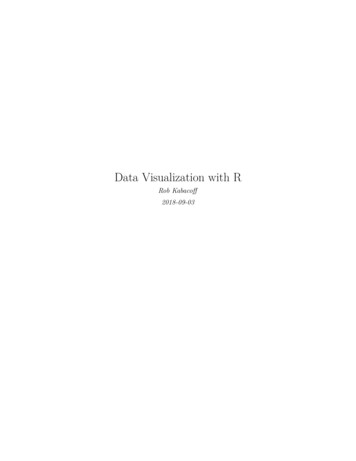
2.1. A WORKED EXAMPLE27colors are more attractive (IMHO).Here is a question. Is the relationship between experience, wages and sex the same for each job sector? Let’srepeat this graph once for each job sector in order to explore this.2.1.5facetsFacets reproduce a graph for each level a given variable (or combination of variables). Facets are createdusing functions that start with facet . Here, facets will be defined by the eight levels of the sector variable.# reproduce plot for each level of job sectorggplot(data plotdata,mapping aes(x exper,y wage,color sex)) geom point(alpha .7) geom smooth(method "lm",se FALSE) scale x continuous(breaks seq(0, 60, 10)) scale y continuous(breaks seq(0, 30, 5),label scales::dollar) scale color manual(values c("indianred3","cornflowerblue")) facet wrap( sector)It appears that the differences between mean and women depend on the job sector under consideration.2.1.6labelsGraphs should be easy to interpret and informative labels are a key element in achieving this goal. Thelabs function provides customized labels for the axes and legends. Additionally, a custom title, subtitle,and caption can be added.# add informative labelsggplot(data plotdata,mapping aes(x exper,y wage,color sex)) geom point(alpha .7) geom smooth(method "lm",se FALSE) scale x continuous(breaks seq(0, 60, 10)) scale y continuous(breaks seq(0, 30, 5),label scales::dollar) scale color manual(values c("indianred3","cornflowerblue")) facet wrap( sector) labs(title "Relationship between wages and experience",subtitle "Current Population Survey",caption "source: http://mosaic-web.org/",x " Years of Experience",y "Hourly Wage",color "Gender")

28CHAPTER 2. INTRODUCTION TO GGPLOT2clericalconstmanagmanufotherprofwage 25 20 15 10 5 0 25 20 15 10 5 0sexFMsales0service10 25 20 15 10 5 00102030405001020304050experFigure 2.6: Add job sector, using faceting20304050

2.1. A WORKED EXAMPLE29Relationship between wages and experienceCurrent Population SurveyclericalconstmanagmanufotherprofHourly Wage 25 20 15 10 5 0 25 20 15 10 5 0GenderFMsales0service1020304050 25 20 15 10 5 00102030405001020304050Years of Experiencesource: http://mosaic web.org/Now a viewer doesn’t need to guess what the labels expr and wage mean, or where the data come from.2.1.7themesFinally, we can fine tune the appearance of the graph using themes. Theme functions (which start withtheme ) control background colors, fonts, grid-lines, legend placement, and other non-data related featuresof the graph. Let’s use a cleaner theme.# use a minimalist themeggplot(data plotdata,mapp

# import data from a comma delimited file Salaries - read_csv("salaries.csv") # import data from a tab delimited file Salaries - read_tsv("salaries.txt") These function assume that the first line of data contains the variable names, values are separated by commas or tabs respectively, and that missing data are represented by blanks.