WIXLIB

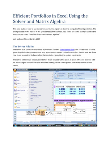
Efficient Portfolios in Excel Using theSolver and Matrix AlgebraThis note outlines how to use the solver and matrix algebra in Excel to compute efficient portfolios. Theexample used in this note is in the spreadsheet 3firmExample.xlsx, and is the same example used in thelecture notes titled “Portfolio Theory with Matrix Algebra”.Last updated: November 24, 2009The Solver Add InThe solver is an Excel Add‐In created by Frontline Systems (www.solver.com) that can be used to solvegeneral optimization problems that may be subject to certain kinds of constraints. In this note we showhow it can be used to find portfolios that minimize risk subject to certain constraints.The solver add‐in must be activated before it can be used within Excel. In Excel 2007, you activate add‐ins by clicking on the office button and then clicking on the Excel Options box at the bottom of themenu.

This opens the Excel options dialogue box. Click Add‐Ins, which displays the available Add‐Ins for Excel.Make sure the Solver Add‐In is an Active Application Add‐In.Matrix Algebra in ExcelExcel has several built‐in array formulas that can perform basic matrix algebra operations. The mainfunctions are listed in table belowArray FunctionMINVERSEMMULTTRANSPOSEDescriptionCompute inverse of matrixMatrix multiplicationCompute transpose of matrixTo evaluate an array function in Excel, you must use the magic key stoke combination: CTRL ‐ SHIFT ‐ ENTER (hold down all three keys at once then release).Example DataIn the Data tab of the spreadsheet 3firmExample.xls is the example monthly return data on three assets:Microsoft, Nordstrom and Starbucks. The monthly means and covariance matrix of the returns arecomputed and these are referenced as the input data on the portfolio tab as illustrated in the screenshot below.

In the spreadsheet, cells colored light blue contain input data (fixed data not created by some formula)and cells colored tan contain output data (data created by applying some formula). Also, some cells areexplicitly named. For example the range of cells B3:B5 is named muvec. If these cells are highlightedthen muvec will appear in the Name Box in the upper left hand corner of the spreadsheet. Similarly, therange of cells E3:G5 is named sigma. For matrix algebra calculations, it is convenient to use namedranges in array formulas.The Global Minimum Variance PortfolioThe global minimum variance portfolio solves the optimization problemmin σ p2 ,m m′Σm s.t. m′1 1mThis optimization problem can be solved easily using the solver with matrix algebra functions. Thescreen shot of the portfolio tab below shows how to set‐up this optimization problem in Excel.

The range of cells D10:D12 is called mvec and will contain the weights in the minimum variance portfolioonce the solver is run and the solution to the optimization problem is found. Before the solver is to berun, these cells should contain an initial guess of the minimum variance portfolio. A simple guess forthis vector whose weights sum to one is mmsft 0.3, mnord 0.3, msbux 0.4.To use the solver, a cell containing the function to be maximized or minimized must be specified. Here,this cell is F10 which contains the array formula{ MMULT(TRANSPOSE(mvec),MMULT(sigma,mvec))}2which evaluates the matrix algebra formula for the variance of a portfolio: σ p ,m m′Σm . Notice thatthe formula is surrounded by curly braces {}. This indicates that CTRL ‐ Shift ‐ Enter was used toevaluate the formula so that it is to be interpreted as an array formula. If you don’t see the curly bracesthen the formula will not be evaluate correctly. We also need a cell to contain a formula that will beused to impose the constraint that the portfolio weights sum to one: m′1 mmsft mnord msbux 1.This formula is specified in cell E10 as SUM(mvec)The solver add‐in is located on the data tab of the top menu ribbon in the right hand corner. To run thesolver, click the cell containing the formula you want to optimize (cell F10, and named sig2px) and thenclick on the solver button. This will open up the solver dialogue box as shown below.

The field named Set Target Cell must contain either the name or the reference to the cell containing theformula to optimize. You have three choices for the type of optimization: Max, Min and Value of. Here,we want to minimize the portfolio variance so Min should be selected. Next, we must specify the cellscontaining the variables which are being optimized. These are specified in the By Changing Cells field.Here, we can type in the name mvec or specify the range of cells D10:D12. Finally, we must Add theconstraint that the weights sum to one. We do this by clicking the Add button, which opens the AddConstraint dialogue box show below.The Cell Reference contains the cell (E10) that has the formula for the constraintm′1 mmsft mnord msbux 1. We specify the value of the constraint, 1, in the Constraint field. Onceeverything is filled in, click OK to go back to the solver dialogue. The complete dialogue should look likeone shown below.

To run the solver, click the Solve button. The computation is generally very fast. If successful, you shouldsee the following dialogue boxThe message “Solver found a solution. All constraints and optimality conditions are satisfied” means thatthe first and second order conditions for a minimum are satisfied. Click the Keep Solver Solution optionbutton and then click OK. Your spreadsheet should look like the one below.

The global minimum variance portfolio has 44% in Microsoft, 36% in Nordstrom and 19% in Starbucks.The expected return on this portfolio is given in cell C13 (called mupx) and is computed using theformula μ p ,m m′μ . The Excel array formula is{ MMULT(TRANSPOSE(mvec),muvec)}The portfolio standard deviation in cell C14 is the square root of the portfolio variance, sig2px, in cellF10.Minimum Variance Portfolio subject to Target Expected ReturnA minimum variance portfolio with target expected return equal to μ0 solves the optimization problemmin σ p2 , y y ′Σy s.t. y′μ μ0 and y′1 1yThis optimization problem can also be easily solved using the solver with matrix algebra functions. Thescreenshot below shows how to set‐up this optimization problem in Excel where the target expectedreturn is the expected return on Microsoft (4.27%).

The range of cells K10:K12 is called yvec and will contain the weights in the efficient portfolio once thesolver is run and the solution to the optimization problem is found. Before the solver is to be run, thesecells should contain an initial guess of the minimum variance portfolio. A simple guess for this vectorwhose weights sum to one is ymsft 0.3, ynord 0.3, ysbux 0.4. The cell containing the formula for2portfolio variance, σ p , y y′Σy , is in cell O10 which contains the array formula{ MMULT(TRANSPOSE(yvec),MMULT(sigma,yvec))}We also need two additional cells to contain formulas that will be used to impose the constraints thatthe portfolio expected return is equal to the target return, μ p , y y ′μ μ0 , and that the portfolioweights sum to one, y ′1 ymsft ynord ysbux 1. These formulas are specified in cells L10 and N10,which contain the Excel formulas SUM(yvec) and { MMULT(TRANSPOSE(yvec),muvec)}, respectively.To run the solver, click cell O10 (called sig2py) and then click on the solver button. Make sure the solverdialogue box is filled out to look like the one below.

Notice that there are now two constraints specified. The first one imposes y ′1 ymsft ynord ysbux 1 ,and the second one imposes μ p , y y ′μ μ0 μ msft 0.0475 . To run the solver, click the Solvebutton. You should see a dialogue box that says that the solver found a solution and that all optimalityconditions are satisfied. Keep the solution and click OK. Your spreadsheet should look like the onebelow.The efficient portfolio has weights ymsft 0.83, ynord 0.09, ysbux 0.26. Notice that Nordstrom issold short in this portfolio because it has a negative weight. The expected return on this portfolio isequal to the target expected return (see cell N10 named mupy) and the weights sum to one. Notice thatthe standard deviation of this portfolio (see cell P10) is smaller than the standard deviation of Microsoft(see cell C3).Computing the Efficient Frontier of Risky AssetsThe efficient frontier of risky assets can be constructed from any two efficient portfolios. A naturalquestion to ask is which two efficient portfolios should be used? I find that the following two efficientportfolios leads to the easy creation of the efficient frontier:1. Efficient portfolio 1: global minimum variance portfolio2. Efficient portfolio 2: efficient portfolio with target expected return equal to the highest averagereturn among the assets under consideration.For the current example, the asset with the highest average return is Microsoft (average return is 4.27%)and we already computed the efficient portfolio with target expected return equal to the average returnon Microsoft.Given any two efficient portfolios with weight vectors m and y the convex combinationz α m (1 α ) y

for any constant α is also an efficient portfolio. The expected return and variance of this portfolio areμ p , z α μ p ,m (1 α ) μ p , yσ p2 , z α 2σ p2 ,m (1 α ) 2 σ p2 , y 2α (1 α )σ my,where the covariance between the returns on portfolios m and y is computed using σ my m′Σy . Tocreate the efficient frontier, create a grid of α values starting at 1 and decrease in increments of 0.1.Use as many values in the grid as necessary to make a nice plot.A screenshot of the part of the spreadsheet to create these portfolios is shown below.Consider the first convex combination with α 1 . This portfolio is the global minimum varianceportfolio. The cell P20 contains the formula N20*mupx O20*mupy for the expected portfolio return,and the cell Q20 contains the formula N20 2*sig2px O20 2*sig2py 2*N20*O20*sigmaxy for theportfolio variance. The covariance term sigmaxy is computed in the cell R9 (not shown) which containsthe array formula { MMULT(MMULT(TRANSPOSE(mvec),sigma),yvec)}. The cells S20:U20 give theweights in the convex combination computed using the array formula{ TRANSPOSE(N20*D10:D12 O20*K10:K12)}.

The efficient frontier can be plotted by making a scatter plot with the expected return values (cellsP20:P50) on the y‐axis and the standard deviation values (cells R20:R50) on the horizontal axis.Computing the Tangency PortfolioThe tangency portfolio is the portfolio of risky assets that has the highest Sharpe’s slope. This portfoliocan be found by solving the optimization problemmaxtt′μ rf( t′Σt )1/2s.t. t′1 1This optimization problem can also be easily solved using the solver with matrix algebra functions. Thescreenshot below shows how to set‐up this optimization problem in Excel.The range of cells D33:D35 is called tvec and will contain the weights in the tangency portfolio once thesolver is run and the solution to the optimization problem is found. Before the solver is to be run, thesecells should contain an initial guess of the minimum variance portfolio. A simple guess for this vectorwhose weights sum to one is tmsft 0.3, tnord 0.3, t sbux 0.4. The computation of Sharpe’s slope isbroken down into two pieces. The first piece is the numerator of Sharpe’s slope, μ p ,t rf t ′μ rf ,and is computed in cell F33 using the array formula { MMULT(TRANSPOSE(tvec),muvec)‐rf}. The second2piece is the square of the denominator of Sharpe’s slope, σ p ,t t′Σt , and is computed in cell G33 usingthe array formula { MMULT(TRANSPOSE(tvec),MMULT(sigma,tvec))}. Finally, Sharpe’s slope isevaluated in cell H33 using the formula F33/SQRT(G33). This is the cell that is passed to the solver.To run the solver, click cell H33 and then click on the solver button. Make sure the solver dialogue box isfilled out to look like the one below.