Transcription
Appendix 4Using Analytic Solver Platform for EducationA4.1. BACKGROUNDPurchasers of this book have the option to download a Windows-based software package calledAnalytic Solver Platform for Education (ASPE), which has all the functionality of thecommercial product Analytic Solver Platform but with restrictive limits on the size ofoptimization problems and "educational use" watermarks on charts. All the examples andexercises in this book can be solved within the limits of ASPE. In this Appendix, we introduceASPE software and provide details on its use.ASPE was developed by the same team that created Excel’s Solver, and it will accommodate allmodels built with Excel’s Solver. However, ASPE is a more powerful version of Excel’s Solverand relies on a different user interface. ASPE is an integration of several software packages,including Risk Solver Platform for Education (RSPE), which is the optimization softwareincluded in ASPE. For the purposes of optimization, references to ASPE or RSPE areinterchangeable.A4.2. INSTALLING ASPEIf you’ve purchased this book and you are a student enrolled in a university course, you candownload and install the software and use ASPE for a full semester (140 days) at no charge. Todo so, visit www.solver.com/welcome-students, fill out the form on this page, and click thebutton to register and download. To complete the form, you’ll need two pieces of information: aTextbook Code, which is BOMS3, and a Course Code, which your instructor can obtain foryou from Frontline Systems, Inc.1If you’ve purchased this book for self-study but you’re not enrolled in a university course, youhave two options: (1) Visit www.solver.com and register on the forms presented there, downloadand install the software, and use ASP (the full commercial product with much higher size limits)on a free trial, which is currently limited to 15 days; or (2) Contact Frontline Systems at 775831-0300 or info@solver.com and request a Course Code that will allow you to use ASPE for140 days. As long as you’re using the software for learning rather than production use, thecompany’s current policy is to routinely grant these licenses.The software works with Excel 2007, Excel 2010 and Excel 2013, but if you are using the 64-bitversion of Excel, be sure to download and run the Setup program for 64-bit Analytic SolverPlatform, named SolverSetup64.exe. In all other cases, you’ll download and runSolverSetup.exe.1For longer-term licenses, course instructors should contact Frontline Systems at 775-831-0300 or info@solver.com
Running the Setup program is straightforward, but you’ll need to pay attention to three prompts:1. You’ll be asked for an installation password. This will be emailed to you, at the emailaddress you give when you fill out the registration form.2. You’ll be asked for a license activation code. This appears in the same email as theinstallation password; it determines whether you’ll be using full ASP for 15 days, ASPEfor 140 days, or something else.3. You’ll be asked whether you want to run initially as full Analytic Solver Platform, or asubset product. There are several choices, but for use with this book, the recommendedselection is Risk Solver Platform. The user interface for optimization is the same inAnalytic Solver Platform, Risk Solver Platform, and Premium Solver Platform. (You canchange this selection later, using Help – Change Product on the ASPE/RSPE Ribbon.)For simplicity, the instructions here refer just to ASPE.To uninstall the software, you can either re-run SolverSetup.exe, or use the WindowsAdd/Remove Programs feature.A4.3. THE ASPE USER INTERFACEIn order to illustrate the use of ASPE, we return to Example 1.1 in Chapter 1. The optimizationproblem is to find a price that maximizes quarterly profit contribution. An algebraic statement ofthe problem is as follows:Maximizesubject toz (x – 40) yy 5x 800(objective)(constraint)This form of the model corresponds to Figure 1.2 (reproduced here as Figure A4.1), whichcontains two decision variables (x and y, or price and demand) and one constraint on the decisionvariables. The spreadsheet model is ready for optimization.
Figure A4.1. Model for Example 1.1To start, we select the Risk Solver Platform tab and click on the Model icon (on the leftside of its ribbon). This step opens the task pane on the right-hand side of the Excel window. Thetask pane contains four tabs: Model, Platform, Engine, and Output. Initially, the Model tabdisplays a window listing several components of the software, including Optimization. In FigureA4.2, we have expanded the Optimization entry on the Model tab. As we specify the elements ofour model, they are recorded in the folder icons of this window. At the top of the model tab, fiveicons appear: Green “plus” sign, to Add model specificationsRed “delete” sign, to Remove specificationsOrange paired sheets with small blue arrows, to Refresh the display after changesGreen checked sheet, to Analyze the modelGreen triangle, to Solve the specified optimization problemTo specify the model we first select the decision cells (C9:C10) and then on the drop-down menuof the Add icon, we select Add Variable. The range C 9: C 10 immediately appears in theModel window, in the folder for Normal Variables. (Another way to accomplish this step withoutthe drop-down menu is to highlight the Normal Variables folder icon and click the Add icon.)
Figure A4.2. Model tab on the initial task paneNext, we select the objective cell (C16) and on the drop-down menu of the Add icon, selectObjective. The cell address C 16 immediately appears in the Model window, in the folder forObjective. By default, the specification assumes that the objective is to maximize this value. (Wecan also implement this step by highlighting the Objective folder and simply clicking the Addicon.)Next, we select the left-hand side of the constraint (C13) and on the drop-down menu of theAdd icon, select Add Constraint. (Alternatively, we can highlight the Normal Constraints foldericon and click the Add icon.) The Add Constraint window appears, with the cell address C 13in the Cell Reference box, as shown in Figure A4.3. On the drop-down menu to its right, weselect “ ” and enter E13 in the Constraint box (or, with the cursor in the box, select cell E13.).Figure A4.3. Add Constraint window
As mentioned in Chapter 1, one of our design guidelines for Solver models is to reference a cellcontaining a formula in the Cell Reference box and to reference a cell containing a number in theConstraint box. The use of cell references keeps the key parameters visible on the spreadsheetrather than in the less accessible windows of Solver’s interface. Ideally, another person wouldnot have to examine the task pane to understand the model. (Although Solver permits us to enternumerical values directly into the Constraint box, this form is less effective for communicationand complicates sensitivity analysis. It would be reasonable only in special cases where themodel structure is obvious from the spreadsheet and where we expect to perform no sensitivityanalyses for the corresponding parameter.)Finally, we press OK and observe that the task pane displays the model’s specification, asshown in Figure A4.4. In summary, our model specification is the following:Objective:Variables:Constraint:C16 (maximize)C9:C10C13 E13If necessary, we can edit specifications by double-clicking on the corresponding cell address as itappears on the Model tab.Figure A4.4. Model specification
This model is simple enough that we need not address the information on the Platform tab.(However, it is generally a good idea to set the Nonsmooth Model Transformation option toNever.) At the top of the Engine tab, we observe the default selection of the Standard LSGRGNonlinear Engine, which we refer to as the nonlinear solver. (To ensure this selection, weuncheck the box for Automatically Select Engine.) This solution algorithm is appropriate for ouroptimization problem, and we do not need to address most of the other information on the tab.However, one of the options is important.Although we may guess that the optimal price is a positive quantity, the model as specifiedpermits the price decision to be negative. Such an outcome would not make sense in thisproblem, so it may be a good idea to limit the model to nonnegative prices. In fact, virtually allof the models in this book involve decision variables that make practical sense only when theyare nonnegative, so we will impose this restriction routinely. On the Engine tab of the task pane,we find the Assume Non-Negative option in the General group and change it to True, using thedrop-down menu on the right-hand side, as shown in Figure A4.5.Figure A4.5. Setting the Assume Non-Negative optionFinally, we proceed to the Output tab (or return to the Model tab) and click the Solve icon. Solversearches for the optimal price and ultimately places it in the price cell. In this case, the optimalprice is 100, and the corresponding quarterly profit contribution is 18,000, as discussed inChapter 1.Meanwhile, the Output tab’s window displays the solution log for the optimization run.(The detail in this log is controlled by the Log Level option on the Platform tab, but the default
setting of Normal is usually adequate.) The most important part of the log is the Solver Resultsmessage, which in this case states:Solver found a solution. All constraints andoptimality conditions are satisfied.This optimality message, which is repeated at the very bottom of the task pane, tells us that noproblems arose during the optimization, and Solver was able to find an optimal solution.We have used Example 1.1 to introduce the user interface of ASPE. The task pane containsmany user-selected options that are not a concern in this problem. Later in this appendix, wecover many of these settings and discuss when they become relevant. We also discuss thevariations that can occur in optimization runs. For example, depending on the initial values of thedecision variables, the nonlinear solver may generate the following result message in the solutionlog:Solver has converged to the currentsolution. All constraints are satisfied.This convergence message indicates that Solver has not been able to confirm optimality. Asmentioned in Chapter 1, this condition occurs because of numerical issues in the solutionalgorithm, and the resolution is to rerun Solver from the point where convergence occurred.Normally, one or two iterations are sufficient to produce the optimality message. We discusssome other result messages later.To minimize an objective function instead of maximizing it, we return to the Model tab ofthe task pane and double-click on the entry in the Objective folder. The Change Objectivewindow appears, as shown in Figure A4.6, and we can select the button for Min rather than Max.Figure A4.6. Selecting minimization of an objectiveWhen an optimization model contains several decision variables, we can enter them one at atime, creating a list of Normal Variables in the task pane, each with its own checked box. Moreconveniently, we can arrange the spreadsheet so that all the variables appear in adjacent cells, asin Figure A4.1, and reference their cell range with just one entry in the Normal Variables folder.Because most optimization problems have several decision variables, we save time by placingthem in adjacent cells whenever that’s convenient. This layout also makes the information in thetask pane easier to interpret.
A4.4. SOLVING LINEAR PROGRAMSWhen solving a linear programming problem, we enter the problem specification using the taskpane. This means entering information about the objective function, decision variables, andconstraints, using the elements of the Model tab as described in the previous section. (Lowerbound and upper bound constraints are entered in the same fashion, using the Add Constraintwindow. However, once they are added to the model, they are displayed in the task pane in theBounds section.) After the model information is entered, we move to the Engine tab and set theAssume Non-Negative option to True.At the top of the Engine tab, we uncheck the box for Automatically Select Engine and,from the drop-down menu above it, select Standard LP/Quadratic Engine. This is the name ofthe linear solver in ASPE. (The same algorithm will solve problems with a quadratic objectivefunction; hence its name.) This algorithm is an enhanced version of the linear solver in Excel.Once the settings on the Engine tab are specified, we can run the solution algorithm by movingto the Model tab or the Output tab and clicking the Solve icon. If no difficulties are encountered,the optimality message appears (with a green background) at the bottom of the task pane, withthe optimal solution displayed on the spreadsheet. The optimality message also appears on theOutput tab, formatted as a link. Clicking on this link opens a Help window that explains theoptimality message. The explanation may seem more extensive than necessary, but that’sbecause the same optimality message appears when other solvers (“engines”) are run. Therefore,the explanation covers several different cases that are not a concern when solving linearprograms.As described in Chapter 2, two exceptions can cause difficulties: infeasible constraints andan unbounded objective function. When the model contains inconsistent constraints, Solverdetects the infeasibility and delivers the following result message in the solution log on theOutput tab as well as at the bottom of the task pane:Solver could not find a feasible solution.Whenever this message appears, there must have been an inconsistency in the set of constraints.Chapter 2 contains a discussion about how to address this type of problem. (Keep in mind thatthe infeasibility message appears in the Output tab as a link to a Help window where furtherinterpretation is available.)The second kind of modeling
To start, we select the Risk Solver Platform tab and click on the Model icon (on the left side of its ribbon). This step opens the task pane on the right-hand side of the Excel window. The task pane contains four tabs: Model, Platform, Engine, and Output. Initially, the Model tabFile Size: 735KBPage Count: 16