WIXLIB

OptimizationUsing Analytic Solver PlatformREVIEW BASED ONMANAGEMENT SCIENCE

What We’ll Cover Today Introduction Frontline Systems Session Ι beta training program goals Overview of Analytic Solver Platform (ASP) Linearity and convexity Model building Guided Mode Reports Parametric optimization4/29/2014WE DEMOCRATIZE ANALYTICS2

Frontline Systems Inc. Software Products for: Conventional and Stochastic Optimization Simulation/Risk Analysis Data Mining and Visualization 26 Years in Business (Founded 1988) 7,000 Companies as Customers: Commercial Academic Software vendors 500,000 Users4/29/2014WE DEMOCRATIZE ANALYTICS3

LecturerSima MalekiPhD - Industrial and Systems Engineering (Operations Research) - the Universityof TennesseeFrontline Systems Consulting Lead and Modeling SpecialistExperienceNetwork design, supply chain simulation and optimization, facility location, 3Dlayout optimization, scheduling, and "lean healthcare" resource utilization.4/29/2014WE DEMOCRATIZE ANALYTICS4

Session Ι Online Beta Training GoalsTo familiarize you with the following concepts: Importance of model structure: linearity and convexity Building models in Excel using ASP Using the ASP Guided Mode to analyze and solve the model Reviewing the reports Using parametric optimization techniqueTo empower you to achieve success State of the art tools Online educational training User guides and video demos4/30/2014WE DEMOCRATIZE ANALYTICS5

Business Analytics Techniques Analyze what hashappened Business intelligencequeries/reports Data visualization Data iveAnalytics Use data to segment orclassify customers Use data to predict futurebehavior Data mining ForecastingWE DEMOCRATIZE ANALYTICS Determine the best courseof action to take Optimization Simulation Decision analysisPrescriptiveAnalytics6

Problem Solving Process It is increasingly important to efficiently use limited resources. Optimization can often improve efficiency with no capital investment.IdentifyProblem4/29/2014Formulate andImplementModelAnalyze ModelWE DEMOCRATIZE ANALYTICSTest ResultsImplementSolution7

Typical Optimization ApplicationsStaff ngBlendingTransportationIndustryFinanceFunctional AreaAgricultureMedia planningSupply chainHealthInventory optimizationMiningVendor selectionDefensePortfolio optimizationForestry4/29/2014Capacity planningProduct mixWE DEMOCRATIZE ANALYTICS8

Frontline SolversOptimization Software1 Million Linear100,000 NonlinearConventionalOptimizationPlug-in Solver EnginesMonte CarloSimulation &Decision TreesStochastic &RobustOptimizationForecastingData MiningAnalytic Solver Platform8,000 Linear1,000 NonlinearRisk Solver PlatformPremium SolverPlatform2,000 Linear500 Nonlinear2004/29/2014Premium Solver ProRisk Solver ProXLMinerSolver BasicWE DEMOCRATIZE ANALYTICS9

Brief Overview ofAnalytic Solver Platform (ASP)RibbonGateway to Analytic Solver Platform’s graphical user interface. Model: to display the Task Pane, defining dimensional models. Optimization Model: to set up optimization models. Simulation Model: to set up simulation models. Parameter: to run multiple optimizations or simulations. Solve Action: to solve optimization or simulation model. Analysis: to analyze the results, create reports and charts.4/29/2014WE DEMOCRATIZE ANALYTICS10

Brief Overview ofAnalytic Solver Platform (ASP)Ribbon Tools: to create decision trees, fit distributions, examine simulation or optimization results. Options: to set options for optimization, simulation, charts and graphs. Help: to display online Help, use Live Chat, control Guided Mode, open examples or an onlinetutorial, access User and Reference Guides, and check the license status.4/29/2014WE DEMOCRATIZE ANALYTICS11

Brief Overview of ASPTask Pane Model button: to display or hide the Task Pane. Model tab: to view the model in outline form, see results of model diagnosis, andoptionally edit model elements in place. Platform tab: to view or change Platform options. Engine tab: to select a Solver Engine and set its options. Output tab: to view a log of solution messages, or a chart of the objective values.4/29/2014WE DEMOCRATIZE ANALYTICS12

Example – Problem Definition A company manufactures and sells two models of hot tubs: the Aqua-Spa and the Hydro-Lux. Aqua-Spa – needs 9 hours of labor, 12 feet of tubing, and 1 pump and generates 350 profit. Hydro-Lux – needs 6 hours of labor, 16 feet of tubing, and 1 pump and generates 300 profit. Company expects to have 200 pumps, 1,566 labor hours, 2,880 feet of tubing. Managerial decision: how many Aqua-Spas and Hydro-Luxes should be produced to maximize theprofit during the next production cycle?4/29/2014ProductsAqua-SpaHydro-LuxTotal AvailabilityLabor Hours961566Tubing Material12162880Pump11200Profit Margin350300MaximizationWE DEMOCRATIZE ANALYTICS13

Examples of Variables,Constraints, and ObjectivePortfolio optimization Variables: amounts invested in different assets Constraints: budget, max. or min. investment per asset, minimum return Objective: overall risk or return variancePower generation Variables: number of generating units, output rate, height of reservoir, Constraints: demand, generator limit Objective: operating, fuel cost, power consumptionProcess manufacturing Variables: raw materials allocated to production processes Constraints: max. or min. outputs, blend specifications Objective: profit or cost of final products4/29/2014WE DEMOCRATIZE ANALYTICS14

Mathematical Optimization Mathematical optimization problem ���𝑖𝑧𝑒 𝑓0 𝑥𝑆𝑢𝑏𝑗𝑒𝑐𝑡 𝑡𝑜 𝑓𝑖 𝑥 𝑏𝑖 ,𝑖 1, , 𝑚ℎ𝑖 𝑥 0,𝑖 𝑚 1, , 𝑀Decision variables: 𝑥 (𝑥1 , , 𝑥𝑛 ):Objective function: 𝑓0Constraint functions: 𝑓𝑖 and ℎ𝑖 for 𝑖 1, , 𝑀Feasible solution: 𝑥 that satisfies all the constraints.Optimal solution: 𝑥 that has the largest/smallest value of 𝑓0 among all possible𝑥 that satisfy the constraints.4/30/2014WE DEMOCRATIZE ANALYTICS15

Example – Problem Formulation Decision variables: number of Aqua-Spas 𝑋1Hydro-Luxes 𝑋2 Objective function to max. profit: 𝑀𝑎𝑥 350𝑋1 300𝑋2 Constraints:Total available labor hours:9𝑋1 6 𝑋2 1566Total available Tubing Material: 12𝑋1 16𝑋2 2880Total pumps:1𝑋1 1 𝑋2 200Bounds on variables:𝑋1 ,𝑋2 tyLabor Hours961566Tubing Material12162880Pump11200Profit Margin350300MaximizationWE DEMOCRATIZE ANALYTICS16

Example – Spreadsheet Implementation Decision variables: number of Aqua-Spas 𝑋1 Spreadsheet Cells: Objective function to max. profit: Spreadsheet Cell:4/30/2014Hydro-Luxes 𝑋2𝑩𝟑𝑪𝟑𝑀𝑎𝑥 350𝑋1 300𝑋2𝐄𝟒 𝐁𝟒 𝐁𝟑 𝐂𝟒 𝐂𝟑 𝐒𝐔𝐌𝐏𝐑𝐎𝐃𝐔𝐂𝐓(𝐁𝟒: 𝐂𝟒, 𝐁𝟑: 𝐂𝟑)WE DEMOCRATIZE ANALYTICS17

Model Structure Matters! Frontline Solvers can optimize any optimization model defined in Excel, however speedand solution quality depend heavily on the formulas you use. This is intrinsic; independent of any optimization software. A linear model will solve quickly, to large scale, and yields a proven optimal solution. A model with IF or LOOKUP functions will solve many times more slowly, cannot be verylarge scale, and yields only a “better” solution. Feasibility or infeasibility can be proven only for convex models.4/29/2014WE DEMOCRATIZE ANALYTICS18

Linear, Non-Linear, Non-SmoothLinear: SUM(A1:A10)Non-linear: A1*A1Non-smooth: IF(A1 25, A1, 0)Easiest/FastestSlowerHardest/Slowest4/29/2014WE DEMOCRATIZE ANALYTICS19

Beyond Linearity: Convexity The key property of functions of the variables that makes aproblem “easy” or “hard” to solve is convexity. Geometrically, a function is convex if, at any two points x and y,the line drawn from x to y (called the chord from x to y) lies onor above the function. All linear functions are convex. The chord from x to y lies on thefunction.f(x)f(y)xy In a minimization problem, if all constraints and objective areconvex you can be confident of finding a globally optimalsolution even if the problem is very large.4/30/2014WE DEMOCRATIZE ANALYTICS20

Non-Convexity A non-convex function “curves up and down.” SIN(C1)Combinations of non-convex functions create complexshapes that are expensive to search. Non-convex functions can have multiple locally optimalsolutions, making it difficult to find the globally optimal solution. A compromise is to seek a “good,” but not a proven optimalsolution. Even one non-convex function makes the whole model nonconvex, and therefore much harder to solve.4/29/2014WE DEMOCRATIZE ANALYTICS21

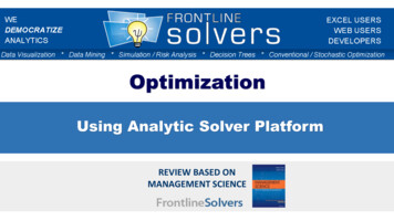
Linear Models: Easy to solve Linear constraints intersect to form a convex region. Optimal solution always lies on the boundary of the feasible region.MaxSubject toA Optimal solutionx2Objective function: 3𝑥1 2𝑥23𝑥1 2𝑥2𝑥1 𝑥2 4,2𝑥1 𝑥2 5, 𝑥1 4𝑥2 2𝑥1 , 𝑥2 0.Feasible Regionx14/29/2014WE DEMOCRATIZE ANALYTICS22

Non-Linear Models: Harder to Solve NLP algorithms begin at a starting point (aninitial feasible solution).Objective functionlevel curves Moves in the direction that improves theobjective function.C Local optimal solution If there is no feasible direction to produce abetter objective function value, it stops.Bx2F A local optimal solution (better than any otherfeasible solutions in its immediate vicinity)might be found instead of global optimalsolution.x1AWE DEMOCRATIZE ANALYTICSsolutionFeasible RegionStarting points4/29/2014GH Global optimalEx123

Non-Smooth Models: Hardest to Solve For a non-smooth model, you should expect only a “good,”not an optimal solution. A systematic search would take exponentially long. Evolutionary algorithm relies on random sampling. Maintains a population of candidate solutions. Makes random changes and combines elements ofexisting solutions to create a new solution. Performs a selection process. Stops and returns a solution when certain heuristic rulesindicate that further progress is unlikely or when itexceeds a limit on computing time.x2FeasibleRegionx1 http://xefer.com/maze-generator4/29/2014WE DEMOCRATIZE ANALYTICS24

Recap – Optimization Solutions Optimal solution – a feasible solution where the objective function reaches its maximum (orminimum) value. Globally optimal solution is one where there are no other feasible solutions with betterobjective function values. A locally optimal solution is one where there are no other feasible solutions “in the vicinity”with better objective function values. The kind of solution the Solver can find depends the formulas you use and the Solver Engine youchoose. Smooth convex: expect a globally optimal solution. Smooth non-convex: usually expect a locally optimal solution. Non-smooth: expect to settle for a “good” solution that may or may not be optimal.4/30/2014WE DEMOCRATIZE ANALYTICS25

Formulas Determine YourModel’s Structure SUM and SUMPRODUCT are common in linear models. IF and LOOKUP functions can be non-smooth/non-convex. ASP can automatically find “problem” formulas in your model. IF functions can sometimes be used: A1 is a decision variable, B1 is a constant parameter IF(A1 10, A1,2*A1) is non-smooth IF(B1 10, A1, 2*A1) is linear4/30/2014WE DEMOCRATIZE ANALYTICS26

Model Building in a SpreadsheetUsing Analytic Solver Platform4/29/201427WE DEMOCRATIZE ANALYTICS

Models in Excel Spreadsheets A well-designed, well documented, and accurate spreadsheet model is a valuabletool in decision making. To build an optimization model in Excel, start with a what-if model, with inputcells for decision variables. Create Excel formulas, copy them across cell ranges, Use Excel’s array formulas, and Excel functions that return array results. Use Excel’s rich facilities to access data in external text files, Web pages, andrelational databases to populate the model.4/29/2014WE DEMOCRATIZE ANALYTICS28