Transcription
Neural Predictor for Neural Architecture SearchWei Wen1,2? , Hanxiao Liu1 , Yiran Chen2 , Hai Li2Gabriel Bender1 , Pieter-Jan Kindermans11Google Brain,2Duke UniversityAbstract. Neural Architecture Search methods are effective but oftenuse complex algorithms to come up with the best architecture. We propose an approach with three basic steps that is conceptually much simpler. First we train N random architectures to generate N (architecture,validation accuracy) pairs and use them to train a regression model thatpredicts accuracies for architectures. Next, we use this regression modelto predict the validation accuracies of a large number of random architectures. Finally, we train the top-K predicted architectures and deploy themodel with the best validation result. While this approach seems simple,it is more than 20 as sample efficient as Regularized Evolution on theNASBench-101 benchmark. On ImageNet, it approaches the efficiency ofmore complex and restrictive approaches based on weight sharing suchas ProxylessNAS while being fully (embarrassingly) parallelizable andfriendly to hyper-parameter tuning.Keywords: Neural Architecture Search, Automated Machine Learning,Graph Neural Networks, NASBench-101, Mobile Models, ImageNet1IntroductionEarly Neural Architecture Search (NAS) methods showed impressive results,allowing researchers to automatically find high-quality neural networks withinhuman-defined search spaces [22, 23, 18, 17]. However, these early methods required thousands of models to be trained from scratch to run a single search,making the methods prohibitively expensive for most practitioners. Thus, algorithms which can improve the sample efficiency are of high value. A second consideration when designing a NAS algorithm is friendliness to hyper-parametertuning. In many existing approaches – such as those based on ReinforcementLearning (RL) [22] or Evolutionary Algorithms (EA) [17], trying out a new setof hyper-parameters for the search algorithm requires us to train and evaluatea new set of neural network from scratch. Ideally, we would be able to train asingle set of neural networks, evaluate them once, and then use the results totry out many different hyper-parameter configurations for the search algorithm.A third design consideration of NAS is full parallelizability (or embarassing parallelizability): existing methods based on RL [22], EA [17] and Bayesian Optimization (BO) [6] are complex to implement, requiring complex coordination?Work done as a Research Intern and Student Researcher in Google Brain.
2W. Wen, H. Liu, Y. Chen, H. Li, G. Bender, P.-J. Kindermansbetween tens or hundreds of workers when collecting reward/fitness/acquisitionduring a search. An fully parallelizable algorithm can avoid this coordinationand accelerate the search when idle computing resources are available. Ideally,we pursue an algorithms with the above merits – sample efficiency, friendlinessto hyper-parameter tuning, and full parallelizability.To design a NAS algorithm possessing the three merits described above,we investigate how well it is possible to do using a combination of two techniques which are ubiquitous in the ML community: supervised learning andrandom sampling. We show that an algorithm that intelligently combines thesetwo approaches can be surprisingly effective in practice. With an infinite compute budget, a very simple but naı̈ve approach to architecture search would beto sample tons of random architectures, train and evaluate each one, and thenselect the architectures with the best validation set accuracies for deployment;this is a straightforward application of the ubiquitous random search heuristic.It is friendly to hyper-parameter tuning and is fully parallelizable. However, theefficiency (computational requirements) of this approach makes it infeasible inpractice. For example, to exhaustively train and evaluate all of the 423, 624 architectures in the NASBench-101 [21], it would take roughly 25 years of TPUtraining time. Only a small number of companies and corporate research labs canafford this much compute, and it is far out of reach for most ML practitioners.Search spaceSample N modelsTrain &78.1%(A small subset)validate75.2%BuildNeuralPredictorTrue accuracy77.9%All/ manyPredictNeuralrandom models Predictor accuracy Search space74.9%Top Train &K validatePick the bestvalidationFig. 1: Building (top) and applying (bottom) the Neural Predictor.One way to alleviate this is to identify a small subset of promising models. Ifthis is done with reasonably high precision (i.e., most models selected are indeedof high quality) then we can train and validate just this limited set of models toreliably select a good one for deployment. To achieve this, the proposed NeuralPredictor uses the following steps to perform an architecture search:(1) Build a predictor by training N random architectures to obtain N(architecture, validation accuracy) pairs. Use this data to train a regressor.(2) Quality prediction using the regression model over a large set of random architectures. Select the K most promising architectures for final validation.(3) Final validation of the top K architectures by training them. Then weselect the architecture with the highest validation accuracy to deploy.The workflow is illustrated in Figure 1. In this setup, the first step is atraditional regression problem where we first generate a dataset of N samplesto train on. The second step can be carried out efficiently because evaluating amodel using the predictor is cheap and parallelizable. The third step is nothing
Neural Predictor for Neural Architecture Search3more than traditional validation where we only evaluate a well curated set ofK models. While the method outlined above might seem straightforward, thissolution is surprisingly effective and satisfies the three goals discussed above:– Efficiency: The Neural Predictor strongly outperforms random search onNASBench-101. It is also about 22.83 times as sample-efficient as RegularizedEvolution – the best performing method in the NASBench-101 paper. TheNeural Predictor can easily handle different search spaces. In addition toNASBench-101, we evaluated it on the ProxylessNAS [5] search space andfound that the predicted architecture is as accurate as ProxylessNAS andclearly better than random search.– Friendliness to hyper-parameter tuning: All hyper-parameters of the regression model are cross validated by the dataset collected just once in step (1).The cost of tuning those hyper-parameters is small because the predictormodel is small.– Full parallelizability: The most computationally intensive components of themethod (training N models in step (1) and K models in step (3)) aretrivially parallelizable when sufficient computation resources are available.Furthermore, the architecture selection process uses two of the most ubiquitous tools from the ML toolbox: random sampling and supervised learning. Incontrast, many existing NAS approaches rely on more advanced techniques suchas RL, EA, BO, and weight sharing.2Related WorkNeural Architecture Search was proposed to automate the design of neural networks, by searching models in a design space using techniques such as RL [22],EA [18] or BO [9, 6]. A clear limitation of the early approaches is their computation efficiency. Thus, recent methods often focus on efficient NAS by using weightsharing [2, 4, 16, 5, 14]. As aforementioned, when comparing with previous works,Neural Predictor is friendly to hyper-parameter tuning, conceptually simple andfully parallelizable. Moreover, our Neural Predictor can potentially work as asurrogate model to accelerate accuracy acquisition of architectures during thesearch in RL, EA and BO, or during the candidate architecture evaluation inweight sharing approaches [2].The idea of predictive models of the accuracy, which we use, has been explored in prior works. In [7] an LSTM was used to generate a feature representation of an architecture, which was subsequently used to predict the quality. Theone-shot approach by Bender et al. [2] used a weight sharing model to predict theaccuracy of an individually trained architecture. Baker et al. [1] used predictivemodels to perform early stopping to speed up architecture and hyper-parameteroptimization. NAO [15] used both a learned representation and a predictor tosearch for high quality architecture. PNAS [13] progressively trained a predictorto accelerate the search. A key difference between PNAS and Neural Predictoris that in PNAS the predictor is only a small component in a large traditional
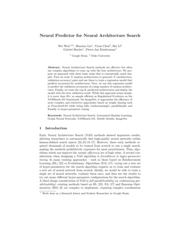
4W. Wen, H. Liu, Y. Chen, H. Li, G. Bender, P.-J. KindermansNAS system. In PNAS, the predictor and the models are trained over time as thearchitectures become more complex. Because of this, the PNAS approach cannotbe completely parallelized. Another popular approach combined a predictor withBayesian Optimization [6]. Unlike above methods, which used ν-SVR/randomforests [1], multi-layer perceptrons [13], LSTMs [15, 7] or Gaussian processes [6],we use a Graph Convolutional Network (GCN) [10] for our regression model.GCNs are naturally permutation-invariant, capturing the intuition that an architecture under different node permutations should have the same predictedaccuracy. Furthermore, we show strong results can be achieved without the useof advanced techniques such as RL, EA, BO or NAO [15], enabling our merits offriendliness to hyper-parameter tuning and full parallelizability. Finally, becausethe effectiveness of NAS has been questioned [12], we include random baselineto show that the search spaces used in this work are meaningful and that whilethe proposed approach is simple, it is clearly better than a random approach.While preparing the final version of this paper, we found a concurrent work [19]which also used a GCN to predict accuracy. However, a node in their graph is amodel in the search space; as the search space is usually huge, their method ishard to scale up. In our design, a graph represents a model and the graph size isapproximately proportional to the number of layers in a model. Therefore, ourNeural Predictor is able to scale to huge search spaces, such as the ProxylessNASImageNet search space with the size of 6.64 1017 .3Neural ,0]3max-poolconv1x11input2[0,0,0,1,0]0, 1, 1, 0, 0, 1[0,1,0,0,0]0, 0, 0, 0, 0, 140, 0, 0, 1, 1, 00, 0, 0, 0, 0, 10, 0, 0, 0, 0, 1[0,1,0,0,0]0, 0, 0, 0, 0, 0adjacency matrixA cell or a network0Operations: [input, conv1x1,[1,0,0,0,0]312040, 0, 0, 0, 0, 01, 0, 0, 0, 0, 01, 0, 0, 0, 0, 00, 0, 1, 0, 0, 00, 0, 1, 0, 0, 01, 1, 0, 1, 1, 0adjacency matrixtransposeconv3x3, max-pool, output]Fig. 2: An illustration of graph and node representations. Left: A neural network architecture with 5 candidate operations per node. Each node is represented by a one-hotcode of its operation. The one-hot codes are inputs of a bidirectional GCN, which takesinto account both the original adjacency matrix (middle) and its transpose (right).The core idea behind the Neural Predictor is that carrying out the actualtraining and validation process is the most reliable way to find the best model.The goal of the Neural Predictor is to provide us with a curated list of promisingmodels for final validation prior to deployment. The entire Neural Predictorprocess is outlined below.
Neural Predictor for Neural Architecture Search5Step 1: Build the predictor using N samples. We train N models toobtain a small dataset of (architecture, validation accuracy) pairs. The datasetis then used to train a regression model that maps an architecture to a predictedvalidation accuracy.Step 2: Quality prediction. Because architecture evaluation using thelearned predictor is efficient and trivially parallelizable, we use it to rapidlypredict the accuracies of a large number of random architectures. We then selectthe top K predicted architectures for final validation.Step 3: Final validation on K samples. We train and validate the topK models in the traditional way. This allows us to select the best model basedon the actual validation accuracy. Even if our predictor is somewhat noisy, thisstep allows us to use a more reliable measurement to select our final architecturefor deployment.Training N K models is by far the most computationally expensive part ofthe Neural Predictor. If we assume a constant compute budget, N and K arekey hyper-parameters which need to be set; we will discuss this next. Note thatthe two most expensive steps (Step 1 and Step 3) are both fully parallelizable.3.1Hyper-parameters in the WorkflowHyper-parameters for model training are always needed if we train a singlemodel in the search space. In this respect the Neural Predictor is no differentfrom other methods. We found that using the same hyper-parameters for allmodels we train is an effective strategy, and was also used in NASBench-101.Trade-off between N and K for a fixed budget: For a given computebudget, the total number of architectures we train and evaluate, N K, mustremain fixed. However, we can trade off between N (the number of samples usedto train the predictor) and K (the number of samples used for final evaluation).If N is too small, the predictor’s outputs will be very noisy and will not providea reliable signal for the search. As we increase N , the predictor will becomemore accurate; however, increasing N requires us to decrease K. If K is small,the predictor must very reliably identify high-quality models from the searchspace. As K increases, we will be able to tolerate larger noise in the predictor,and the predictor’s ability to precisely rank architectures in the search space willbecome less important. Because it is difficult to theoretically predict the optimaltrade-off between N and K, we will investigate this in the experimental setting.To find a lower bound on N we can start with a small number of samples,and iteratively increase N until we observe a good cross-validation accuracy. Thismeans that contrast to some other methods such as Regularized Evolution [17],ENAS [16], NASNet [23], ProxylessNAS [5], there is no need to repeat the entiresearch experiment in order to tune this hyper-parameter. The same applies tothe hyper-parameters and the architecture of the Neural Predictor itself.The hyper-parameters of the Neural Predictor can be optimized bycross-validation using the N training samples. The cost of training a neuralpredictor including the hyper-parameter tuning is negligible compared to thecost of training image models. It takes 25 seconds to train a neural predictor on
6W. Wen, H. Liu, Y. Chen, H. Li, G. Bender, P.-J. KindermansN 172 samples from NASBench-101. The mean (resp. median) training timeof a CIFAR-10 model in NASBench-101 is 32 (resp. 26) minutes. At the costof training two CIFAR-10 models (about one hour), we could try 144 hyperparameter configurations for the neural predictor. In contrast, RL or EA requireus to train more models in order to try out a new hyper-parameter configuration.3.2Modeling by Graph Convolutional NetworksWe tried many options for the architecture of the predictor. We find GraphConvolutional Networks (GCNs) work best. Due to space constraints we willlimit our discussion to GCNs. A comparison against other regression modelsis in the supplementary material. Graph Convolutional Networks (GCNs) aregood at learning representations for graph-structured data [10, 20] such as aneural network architecture. The graph convolutional model we use is based on[10], which assumes undirected graphs. We will modify their approach to handleneural architectures represented as directed graphs.We start with a D0 -dimensional representation for each of the I nodes in thegraph, giving us an initial feature vector V0 RI D0 . For each node we use aone-hot vector representing the selected operation. An example for NASBench101 is shown in Figure 2. The node representation is iteratively updated usingGraph Convolutional Layers. Each layer uses an adjacency matrix A RI Ibased on the node connectivity and a trainable weight matrix Wl RDl Dl 1 :Vl 1 ReLU (AVl Wl ) .(1)Following previous work [10], we add an identity matrix to A (corresponding toself cycles) and normalize it using the node degree.The original GCNs [10] assume undirected graphs. When applied to a directedacyclic graph, the directed adjacency matrix allows information to flow only in asingle direction. To make information flow both ways, we always use the averageof two GCN layers: one where we use A to propagate information in the forwarddirections and another where we use AT to reverse the direction: 1 1Vl 1 ReLU AVl Wl ReLU AT Vl Wl .22Figure 2 shows an example of how the adjacency matrices are constructed (without normalization or self-cycles).GCNs are able to learn high quality node representations by stacking multipleof these layers together. Since we are more interested in the accuracy of the overall network (a global property), we take the average over node representationsfrom the final graph convolutional layer and attach one or more fully connectedlayers to obtain the desired output. Details are provided in the supplementary.4ExperimentsIn this section we will discuss two studies. First we will analyze the NeuralPredictor’s behavior in the controlled environment from NASBench-101 [21].
Neural Predictor for Neural Architecture Search7Afterwards we will use our approach to search for high quality mobile models inthe ProxylessNAS search space [5].4.1NASBench-101Test accuracy %NASBench-101 [21] is a dataset used to benchmark NAS algorithms. The goalis to come up with a high quality architecture as efficiently as possible. Thedataset has the following properties: (1) train time, validation and test accuracyare provided for all 423,624 models in the search space; (2) each model wastrained and evaluated three times. This allows us to look at the variance acrossruns; (3) all models were trained in a consistent manner, preventing biases fromthe implementation from skewing results; (4) NASBench-101 recommends usingonly validation accuracies during a search, and reserving test accuracies for thefinal report; this is important to avoid overfitting.NASBench-101 uses a cell-based NAS [23] on CIFAR-10 [11]. Each cell is aDirected Acyclic Graph (DAG) with up to 7 nodes. There is an input node, anoutput node and up to 5 interior nodes. Each interior node can be a 1 1 convolution (conv1x1), 3 3 convolution (conv3x3) or max-pooling op (max-pool).One example is shown in Figure 2 (left). In each experiment, we use the validation accuracy from a single run 1 as a search signal. The single run is uniformlysampled from these three records. This simulates training the architecture once.Test accuracy is only used for reporting the accuracy on the model that wasselected at the end of a search. For that model we use the mean test accuracyover three runs as the “ground truth” measure of accuracy.Best test modelValidation accuracy %Best validationmodelValidation accuracy %Fig. 3: (Left) Validation vs. test accuracy in NASBench-101. (Right) Zoomed in on thehighly accurate region. Each model (point) is the validation accuracy from a singletraining run. Test accuracies are averaged over three runs. This plot demonstrates thateven knowing the validation accuracy of every possible model is not sufficient to predictwhich model will perform best on the test set.1In the training dataset of our Neural Predictor, this means that each model’s accuracy label is sampled once and fixed across all epochs.
W. Wen, H. Liu, Y. Chen, H. Li, G. Bender, P.-J. 94.4neural predictor w classifierneural predictor w/o classifierregularized evolutionrandom searchoracle94.294.00100020003000The number of samples40005000Test accuracy %95.4Test accuracy %Validation accuracy %893.893.693.4neural predictor w classifierneural predictor w/o classifierregularized evolutionrandom searchoracle93.293.00100020003000The number of samples4000500093.893.693.4neural predictor w classifierneural predictor w/o classifierregularized evolutionrandom searchoracle93.293.00123456Total training time (seconds)781e6Fig. 4: Comparison of search efficiency among oracle, random search, Regularized Evolution and our Neural Predictor (with and without a two stage regressor). All experiments are averaged over 600 runs. The x-axis represents the total compute budgetN K. The vertical dotted line is at N 172 and represents the number of samples(or total training time) used to build our Neural Predictor. From this line on we startfrom K 1 and increase it as we use more architectures for final validation. Theshaded region indicates standard deviation of each search method.Oracle: an upper bound baseline. Under the assumption of infinite compute, a traditional machine learning approach would be to train and validateall possible architectures to select the best one. We refer to this baseline as the“oracle” method. Figure 3 plots the validation versus the test accuracy for allmodels. The model that the oracle method would select based on the validationaccuracy of 95.15% has a test set accuracy of 94.08%. This means that the oracle does not select the model with the highest test set accuracy. Theglobal optimum on the test set is 94.32%. However, since this model cannot befound using extensive validation, one should not expect this model to be foundusing any NAS algorithm. A more reasonable goal is to reliably select a modelthat has similar quality to the one selected by the oracle. Furthermore, it isimportant to realize that even an oracle approach has variance. We havethree training runs for each model, which allows us to run multiple variations ofthe “oracle”. This simulates the impact of random variations on the final result.Averaged over 100 oracle experiments, where in each experiment we randomlyselect one of 3 validation results, the best validation accuracy has a mean 95.13%and a standard deviation 0.03%. The test accuracy has a mean of 94.18% and astandard deviation 0.07%.Random search: a lower bound baseline. Recently, Li et al. [12] questioned whether architecture search methods actually outperform random search.Because this depends heavily on the search space and Li et al. [12] did not investigate the NASBench-101 search space, we need to check this ourselves. Thereforewe replicate the random baseline from NASBench-101 by sampling architectureswithout replacement. After training, we pick the architecture with the highestvalidation accuracy and report its result on the test set. Here we observe that
Neural Predictor for Neural Architecture Search9even when we train and validate 2000 models, which requires a massive computebudget, the gap to the oracle is large (Figure 4). For random search the averagetest accuracy is 93.66% compared to 94.18% for the oracle. This implies thatthere is a large margin for improvement over random search. Moreover, the variance is quite high, with a standard deviation of 0.25%. Finally,evaluating 5000 models in total produces only a small gain over evaluating 2000models at a high computational cost.Regularized evolution: a state of the art baseline. In the NASBench-101paper [21], Regularized Evolution [17] was the best performing method. We replicated those experiments using the open source code and their hyper-parametersettings (available in the supplementary material). Regularized evolution issignificantly better than random as shown in Figure 4. However even after2000 models are trained, it is still clearly worse than the oracle (on average) withan accuracy of 93.97% and a standard deviation of 0.26%.Neural Predictor. Having set our baselines, we now describe the precise Neural Predictor setup and evaluation. The graph representation of a model is a DAGwith up to 7 nodes. Each node is represented by an one-hot code of “[input,conv1x1, conv3x3, max-pool, output]”. The GCN has three Graph Convolutional layers with the constant node representation size D and one hidden fullyconnected layer with output size 128. Finally, the accuracy we need to predictis limited to a finite range. While it is not that common for regression, we canforce the network to make predictions in this finite range by using a sigmoidat the output layer. Specifically, we use a sigmoid function that is scaled andshifted such that its output accuracy is always between 10% and 100%.All hyper-parameters for the predictor are first optimized using cross-validationwhere 13 N samples were used for validation. After setting the hyper-parameters,we use all N samples to train the final predictor. At this point we heuristicallyincrease the node representation size D of the predictor such that the numberof parameters in the Neural Predictor is also 1.5 as large. Specific N and Dvalues and other training details are in the supplementary material. The modelsselected for final evaluation are always trained in the same way, regardless of themethod (baseline or predictor) that selected the model, to ensure fairness.A two stage predictor. Looking at a small dataset of N 172 modelsin Figure 6 (left) during cross-validation,2 we realized that for NASBench-101 atwo stage predictor is needed. The NasBench-101 dataset contains many modelsthat are not stable during training or perform very poorly (e.g. a model withonly pooling operations). The two stage predictor, shown in Figure 5, filtersobviously bad models first by predicting whether each model will achieve anaccuracy above 91%. This allows the the second stage to focus on a narroweraccuracy range. It makes training the regression model easier, which in turn2In our implementation, we split the NASBench-101 dataset to 10, 000 shards andeach shard has 43 samples. The N 172 comes from a random 4 shards.
10W. Wen, H. Liu, Y. Chen, H. Li, G. Bender, P.-J. Kindermansmakes it more reliable. Both stages share the same GCN architecture but havedifferent output layers. A classifier trained on these N 172 models has a lowFalse Negative Rate as shown in Figure 6 (right). This implies that the classifierwill filter out very few actually good GCNRegressoraccuraciesmodelsFig. 5: Neural Predictor onNASBench-101. It is a cascade ofa classifier and a regressor. Theclassifier filters out inaccuratemodels and the regressor predictsaccuracies of accurate models.Fig. 6: The classifier filtering out inaccurate models in NASBench. 172 models (left)are sampled to build the classifier, which istested by unseen data (right).The two stage approach improves the results but is not required. Ifwe only use a single stage, the MSE for the validation accuracy is 1.95 (averagedover 10 random splits). By introducing the filtering stage this reduces to 0.66.In Figure 4 we observe that even without the filtering stage the predictor clearlyoutperforms the random search baseline and regularized evolution. Therefore thetwo stage approach should be seen as a non-essential fine-tuning of the proposedmethod. Using only a single stage is more elegant, but adding the second stagegives additional performance benefits.Results using N 172 (or 0.04% of the search space) for training are shownin Figure 4. We used N 172 models to train the predictor. Then we vary K,the number of architectures with the highest predicted accuracies to be trainedand validated to select the best one. Therefore, “the number of samples” in thefigure equals N K for Neural Predictor. In Figure 4 (left), our Neural Predictor significantly outperforms Regularized Evolution in terms of sample efficiency.The mean validation accuracy is comparable to that of the oracle after about1000 samples. The sample efficiency in validation accuracy transfers well to testaccuracy in terms of both the total number of trained models in Figure 4 (middle) and wall-clock time in Figure 4 (right). After 5000 samples, RegularizedEvolution reaches validation and test accuracies of 95.06% and 94.04% respectively; our predictor can reach the same validation accuracy 12.40 faster andthe same test accuracy 22.83 faster. Another advantage we observe is thatNeural Predictor has small search variance.N vs K and ablation study. We next consider the problem of choosingan optimal value of N when the total number of models we’re permitted totrain, N K, is fixed. Figure 7 summarizes our study on N . A Neural Predictorunderperforms with a very small N (43 or 86), as it cannot predict accuratelyenough which models are interesting to evaluate. Finally, we consider the casewhere N is large (e.g., N 860) but K is small. In this case we clearly seethat the increase in quality of the GCN cannot compensate for the decrease inevaluation budget. Note that in Figure 3 we have shown that some models are
94.494.495.294.294.295.094.094.094.8neural predictor 860neural predictor 344neural predictor 172neural predictor 129neural predictor 86neural predictor 43regularized evolutionrandom searchoracle94.694.494.294.00100020003000The number of samples4000500093.8neural predictor 860neural predictor 344neural predictor 172neural predictor 129neural predictor 86neural predictor 43regularized evolutionrandom searchoracle93.693.493.293.00100020003000The number of samples4000Test accuracy %95.4Test accuracy %Validation accuracy %Neural Predictor for Neural Architecture Search50001193.8neural predictor 860neural predictor 344neural predictor 172neural predictor 129neural predictor 86neural predictor 43regularized evolutionrandom searchoracle93.693.493.293.0012345Total training time (seconds)671e6Fig. 7: Analysis of the trade-off between N training samples vs K final validationsamples in the neural predictor. The x-axis is the total compute budget N K. Thevertical lines indicate different choices for N – the number of training samples and thepoint where we start validating K model
The core idea behind the Neural Predictor is that carrying out the actual training and validation process is the most reliable way to nd the best model. The goal of the Neural Predictor is to provide us with a curated list of promising models for nal validation prior to deployment. The entire Neural Predictor process is outlined below.