WIXLIB

4·Anne Benoit et al.independent tasks for the same data set; it can help minimize the workflow latency.Pipelined-parallelism is used when two dependent tasks in the workflow are being executed simultaneously on different data sets. The goal is to improve thethroughput of the application, possibly at the price of more communications, hencepotentially a larger latency. Pipelined-parallelism was made famous by assemblylines and later reused in processors in the form of the instruction pipeline in CPUsand the graphic rendering pipeline in GPUs.Replicated-parallelism can improve the throughput of the application, becauseseveral copies of a single task operate on different data sets concurrently. This isespecially useful in situations where more computational resources than workflowtasks are available. Replicated-parallelism is possible when reordering the processing of the data sets by one task does not break the application semantics, forinstance when the tasks perform a stateless transformation. A simple example of atask allowing replicated-parallelism would be computing the square root of the dataset (a number), while computing the sum of the numbers processed so far would bestateful and would not allow replicated-parallelism.Finally, data-parallelism may be used when some tasks contain inherent parallelism. It corresponds to using several processors to execute a single task for a singledata set. It is commonly used when a task is implemented by a software librarythat supports parallelism on its own, or when a strongly coupled parallel executioncan be performed.Note that task-parallelism and data-parallelism are inherited from classical workflow scheduling, while pipelined-parallelism and replicated-parallelism are only foundin pipelined workflow scheduling.In a nutshell, the main contributions of this survey are the following: (i) proposinga three-tiered model of pipelined workflow scheduling problems; (ii) structuringexisting work; and (iii) providing detailed explanations on schedule reconstructiontechniques, which are often implicit in the literature.The rest of this paper is organized as follows. Before going into technical details, Section 2 presents a motivating example to illustrate the various parallelismtechniques, task properties, and their impact on objective functions.The first issue when dealing with a pipelined application is to select the rightmodel among the tremendous number of variants that exist. To solve this issue,Section 3 organizes the different characteristics that the target application canexhibit into three components: the workflow model, the system model, and theperformance model. This organization helps position a given problem with respectto related work.The second issue is to build the relevant scheduling problem from the modelof the target application. There is no direct formulation going from the modelto the scheduling problem, so we cannot provide a general method to derive thescheduling problem. However, in Section 4, we illustrate the main techniques onbasic problems, and we show how the application model impacts the schedulingproblem. The scheduling problems become more or less complicated dependingupon the application requirements. As usual in optimization theory, the most basic(and sometimes unrealistic) problems can usually be solved in polynomial time,whereas the most refined and accurate models usually lead to NP-hard problems.ACM Computing Surveys, Vol. V, No. N, January 2014.

A Survey of Pipelined Workflow Scheduling: Models and Algorithms·5Although the complexity of some problems is still open, Section 4 concludes byhighlighting the known frontier between polynomial and NP-complete problems.Finally, in Section 5, we survey various techniques that can be used to solvethe scheduling problem, i.e., to find the best parallel execution of the applicationaccording to the performance criteria. We provide optimal algorithms to solve thesimplest problem instances in polynomial time. For the most difficult instances,we present some general heuristic methods, which aim at giving good approximatesolutions.2.MOTIVATING EXAMPLEIn this section, we focus on a simple pipelined application and emphasize the needfor scheduling algorithms.Consider an application composed of four tasks, whose dependencies form a linearchain: a data set must first be processed by task t1 before it can be processedby t2 , then t3 , and finally t4 . The computation weights of tasks t1 , t2 , t3 and t4(or task weights) are set respectively to 5, 2, 3, and 20, as illustrated in Fig. 1(a).If two consecutive tasks are executed on two distinct processors, then some timeis required for communication, in order to transfer the intermediate result. Thecommunication weights are set respectively to 20, 15 and 1 for communicationst1 t2 , t2 t3 , and t3 t4 (see Fig. 1(a)). The communication weight alongan edge corresponds to the size of the intermediate result that has to be sent fromthe processor in charge of executing the source task of the edge to the processorin charge of executing the sink task of the edge, whenever these two processors aredifferent. Note that since all input data sets have the same size, the intermediateresults when processing different data sets also are assumed to have identical size,even though this assumption may not be true for some applications.The target platform consists of three processors, with various speeds and interconnection bandwidths, as illustrated in Fig. 1(b). If task t1 is scheduled to beexecuted on processor P2 , a data set is processed within 15 5 time units, while the5 0.5 time units (task weightexecution on the faster processor P1 requires only 10divided by processor speed). Similarly, the communication of a data of weight cfrom processor P1 to processor P2 takes 1c time units, while it is ten times faster tocommunicate from P1 to P3 .First examine the execution of the application when mapped sequentially on thefastest processor, P3 (see Fig. 1(c)). For such an execution, there is no communication. The communication weights and processors that are not used are shadedin grey on the figure. On the right, the processing of the first data set (and thebeginning of the second one) is illustrated. Note that because of the dependenciesbetween tasks, this is actually the fastest way to process a single data set. The 1.5. A new data set can be processed oncelatency is computed as L 5 2 3 2020the previous one is finished, hence the period P L 1.5.Of course, this sequential execution does not exploit any parallelism. Since thereare no independent tasks in this application, we cannot use task-parallelism here.However, we now illustrate pipelined-parallelism: different tasks are scheduled ondistinct processors, and thus they can be executed simultaneously on different datasets. In the execution of Fig. 1(d), all processors are used, and we greedily balanceACM Computing Surveys, Vol. V, No. N, January 2014.

·Anne Benoit et al.52t13t220t32t120P31020t3t411P25(b) Platform.15110P113t220110P1t415(a) .251.50.552t13t22020t3t41511P2110processor(c) Sequential execution on the fastest processor.t432520P3P1t2t11100t30.520.5time22.537.5 37.8 37.938.92 2.13523t1t2t320t415110201P2P11processor(d) Greedy execution using all processors.3520P310t4t11t2t3time00.51(e) Resource selection to optimize period.Fig. 1.Motivating example.the computation requirement of tasks according to processor speeds. The performance of such a parallel execution turns out to be quite bad, because several largecommunications occur. The latency is now obtained by summing up all computa31205 20 2 15 10 10 20 38.9, astion and communication times: L 10illustrated on the right of the figure for the first data set. Moreover, the periodis not better than the one obtained with the sequential execution presented previously, because communications become the bottleneck of the execution. Indeed,the transfer from t1 to t2 takes 20 time units, and therefore the period cannot bebetter than 20: P 20. This example of execution illustrates that parallelismshould be used with caution.ACM Computing Surveys, Vol. V, No. N, January 2014.

A Survey of Pipelined Workflow Scheduling: Models and Algorithms·7However, one can obtain a period better than that of the sequential executionas shown in Fig. 1(e). In this case, we enforce some resource selection: the slowestprocessor P2 is discarded (in grey) since it only slows down the whole execution. Weprocess different data sets in parallel (see the execution on the right): within oneunit of time, we can concurrently process one data set by executing t4 on P3 , andanother data set by executing t1 , t2 , t3 (sequentially) on P1 . This partially sequentialexecution avoids all large communication weights (in grey). The communicationtime corresponds only to the communication between t3 and t4 , from P1 to P3 ,1. We assume that communication and computation canand it takes a time 10overlap when processing distinct data sets, and therefore, once the first data sethas been processed (at time 1), P1 can simultaneously communicate the data to P3and start computing the second data set. Finally, the period is P 1. Note thatthis improved period is obtained at the price of a higher latency: the latency has1increased from 1.5 in the fully sequential execution to L 1 10 1 2.1 here.This example illustrates the necessity of finding efficient trade-offs between antagonistic criteria.3.MODELING TOOLSThis section gives general information on the various scheduling problems. It shouldhelp the reader understand the key properties of pipelined applications.All applications of pipelined scheduling are characterized by properties from threecomponents that we call the workflow model, the system model and the performancemodel. These components correspond to “which kind of program we are scheduling”, “which parallel machine will host the program”, and “what are we trying tooptimize”. This three-component view is similar to the three-field notation used todefine classical scheduling problems [Bru07].In the example of Section 2, the workflow model is an application with fourtasks arranged as a linear chain, with computation and communication weights;the system model is a three-processor platform with speeds and bandwidths; andthe performance model corresponds to the two optimization criteria, latency andperiod. We present in Sections 3.1, 3.2 and 3.3 the three models; then Section 3.4classifies work in the taxonomy that has been detailed.3.1Workflow ModelThe workflow model defines the program that is going to be executed; its components are presented in Fig. 2.As stated in the introduction, programs are usually represented as DirectedAcyclic Graphs (DAGs) in which nodes represent computation tasks, and edgesrepresent dependencies and/or communications between tasks. The shape of thegraph is a parameter. Most program DAGs are not arbitrary but instead have somepredefined form. For instance, it is common to find DAGs that are a single linearchain, as in the example of Section 2. Some other frequently encountered structuresare fork graphs (for reduce operations), trees (in arithmetic expression evaluation;for instance in database [HM94]), fork-join, and series-parallel graphs (commonlyfound when using nested parallelism [BHS 94]). The DAG is sometimes extendedwith two zero-weight nodes, a source node, which is made a predecessor of all entrynodes of the DAG, and a sink node, which is made a successor of all exit nodes ofACM Computing Surveys, Vol. V, No. N, January 2014.

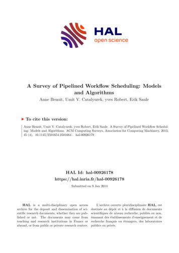
8·Anne Benoit et al.Workflow ExecutionLinear chain, fork, tree,fork-join, series-parallel,general DAGunit, non-unit0 (precedence only),unit, g. 2.The components of the workflow model.the DAG. This construction is purely technical and allows for faster computationof dependence paths in the graph.The weight of the tasks are important because they represent computation requirements. For some applications, all the tasks have the same computation requirement (they are said to be unit tasks). The weight of communications is definedsimilarly, it usually corresponds to the size of the data to be communicated fromone task to another, when mapped on different processors. Note that a zero weightmay be used to express a precedence between tasks, when the time to communicatecan be ignored.The tasks of the program may themselves contain parallelism. This adds a levelof parallelism to the execution of the application, that is called data-parallelism.Although the standard model only uses sequential tasks, some applications featureparallel tasks. Three models of parallel tasks are commonly used (this naming wasproposed by [FRS 97] and is now commonly used in job scheduling for productionsystems): a rigid task requires a given number of processors to execute; a moldabletask can run on any number of processors, and its computation time is given bya speed-up function (that can either be arbitrary, or match a classical model suchas the Amdahl’s law [Amd67]); and a malleable task can change the number ofprocessors it is executing on during its execution.The task execution model indicates whether it is possible to execute concurrentreplicas of a task at the same time or not. Replicating a task may not be possible dueto an internal state of the task; the processing of the next data set depends upon theresult of the computation of the current one. Such tasks are said to be monolithic;otherwise they are replicable. When a task is replicated, it is common to imposesome constraints on the allocation of the data sets to the replicas. For instance, thedealable stage rule [Col04] forces data sets to be allocated in a round-robin fashionamong the replicas. This constraint is enforced to avoid out-of-order completionand is quite useful when, say, a replicated task is followed by a monolithic one.3.2System ModelThe system model describes the parallel machine used to run the program; itscomponents are presented in Fig. 3 and are now described in more details.First, processors may be identical (homogeneous), or instead they can have different processing capabilities (heterogeneous). There are two common models ofheterogeneous processors. Either their processing capabilities are linked by a constant factor, i.e., the processors have different speeds (known as the related modelin scheduling theory and sometimes called heterogeneous uniform), or they are notACM Computing Surveys, Vol. V, No. N, January 2014.

A Survey of Pipelined Workflow Scheduling: Models and Algorithms·9System tero-unrelatedTopologyTypeFully Connected,Structured, Unstructuredhomogeneous,heterogeneousFig. 3.CommunicationCompute &Communicatesingle-port, unboundedmulti-port, bw-boundedmulti-port, k-portoverlap,non-overlapThe components of the system model.speed-related, which means that a processor may be fast on a task but slow onanother one (known as the unrelated model in scheduling theory and sometimescalled completely heterogeneous). Homogeneous and related processors are common in clusters. Unrelated processors arise when dealing with dedicated hardwareor from preventing certain tasks to execute on some machines (to handle licensingissues or applications that do not fit in some machine memory). This decompositionin three models is classical in the scheduling literature [Bru07].The network defines how the processors are interconnected. The topology ofthe network describes the presence and capacity of the interconnection links. It iscommon to find fully connected networks in the literature, which can model busesas well as Internet connectivity. Arbitrary networks whose topologies are specifiedexplicitly through an interconnection graph are also common. In between, somesystems may exhibit structured networks such as chains, 2D-meshes, 3D-torus, etc.Regardless of the connectivity of the network, links may be of different types. Theycan be homogeneous – transport the information in the same way – or they canhave different speeds. The most common heterogeneous link model is the bandwidthmodel, in which a link is characterized by its sole bandwidth. There exist othercommunication models such as the delay model [RS87], which assumes that allthe communications are completely independent. Therefore, the delay model doesnot require communications to be scheduled on the network but only requires theprocessors to wait for a given amount of time when a communication is required.Frequently, the delay between two tasks scheduled on two different processors iscomputed based on the size of the message and the characteristics (latency andbandwidth) of the link between the processors. The LogP (Latency, overhead, gapand Processor) model [CKP 93] is a realistic communication model for fixed sizemessages. It takes into account the transfer time on the network, the latency of thenetwork and the time required by a processor to prepare the communication. TheLogGP model [AISS95] extends the LogP model by taking the size of the messageinto account using a linear model for the bandwidth. The latter two models areseldom used in pipelined scheduling.Some assumptions must be made in order to define how communications takeplace. The one-port model [BRP03] forbids a processor to be involved in morethan one communication at a time. This simple, but somewhat pessimistic, modelis useful for representing single-threaded systems; it has been reported to accuratelyACM Computing Surveys, Vol. V, No. N, January 2014.

10·Anne Benoit et al.model certain MPI implementations that serialize communications when the messages are larger than a few megabytes [SP04]. The opposite model is the multi-portmodel that allows a processor to be involved in an arbitrary number of communications simultaneously. This model is often considered to be unrealistic since somealgorithms will use a large number of simultaneous communications, which induceslarge overheads in practice. An in-between model is the k-port model where thenumber of simultaneous communications must be bounded by a parameter of theproblem [HP03]. In any case, the model can also limit the total bandwidth that anode can use at a given time (that corresponds to the capacity of its network card).Finally, some machines have hardware dedicated to communication or use multithreading to handle communication; thus they can compute while using the network. This leads to an overlap of communication and computation, as was assumedin the example of Section 2. However, some machines or software libraries are stillmono-threaded, and then such an overlapping is not possible.3.3Performance ModelThe performance model describes the goal of the scheduler and tells from two validschedules which one is better. Its components are presented in Fig. 4.The most common objective in pipelined scheduling is to maximize the throughput of the system, which is the number of data sets processed per time unit. Inpermanent applications such as interactive real time systems, it indicates the load

nature of the systems. The main focus of this paper is a special class of workflow scheduling that we call pipelined workflow scheduling (or in short pipelined scheduling). Indeed, we focus on the scheduling of applications that continuously operate on a stream of data sets, which are processed by a given wokflow, and hence the term pipelined.