WIXLIB

Visualizing Data with Graphs and MapsChapter 1In the same way as working time, the trigger line is displayed in simple graphs withno way to disable it.There was another checkbox that could make this graph different from a simplegraph—Show legend. Let's see what a graph would look like with these three optionsdisabled. In the graph configuration, unmark Show legend, Show working time, andShow triggers, and then click on Update.When reconfiguring graphs, it is suggested using two browser tabsor windows, keeping Monitoring Graphs open in one, and thegraph details in the Configuration section in the other. This way,you will be able to refresh the monitoring section after makingconfiguration changes, saving a few clicks back and forth.Open this graph in the monitoring section again:Sometimes, all that extra information can take up too much space—especially thelegend, if you have lots of items on a graph. For custom graphs, we may hide it. Reenable these checkboxes in the graph configuration and save the changes by clickingon the same Update button.Graph item functionWhat we have now is quite similar to the simple graphs, although there's one notabledifference when the displayed period is longer; simple graphs show three differentlines, with the area between them filled, while our graph has a single line only (thedifference is easier to spot when the displayed period approaches 3 days). Can weduplicate that behavior? Go to Configuration Templates, click on Graphs next toC Template Linux, and then click on CPU load in the Name column to open theediting form. Take a closer look at the FUNCTION drop-down in the Items section:[ 10 ]

Visualizing Data with Graphs and MapsChapter 1Currently, we have avg selected, which simply draws average values. The otherchoices are quite obvious – min and max, except the one that looks suspicious, all.Select all, and then click on Update. Again, open Monitoring Graphs and makesure that CPU load is selected in the Graph drop-down:The graph now has three lines, representing minimum, maximum, and averagevalues for each point in time, although in this example, the lower line is always atzero.The default is average, since showing three lines with the colored area when there aremany items on a graph would surely make the graph unreadable. On the other hand,even when average is chosen, the graph legend shows minimum and maximumvalues from the raw data, which are used to calculate the average line. This can resultin a situation where the line does not go above 1, but the legend says that themaximum is 5. In such a case, almost always, the raw values can be seen by zoomingin on the area that has them, but such a situation can still be confusing.[ 11 ]

Visualizing Data with Graphs and MapsChapter 1Two y-axesWe have now faithfully replicated a simple graph (well, the simple graph uses greenfor average values, while we use another color, which is a minor difference). Whilesuch an experience should make you appreciate the availability of simple graphs,custom graphs would be quite useless if that was all we could achieve with them.Customization such as color, function, and working time displaying can be useful,but they are minor elements. Let's see what else we can throw at the graph. Before weimprove the graph, let's add one more item. We monitored the incoming traffic, butnot the outgoing traffic:1. Go to Configuration Templates, click on Items next toC Template Linux, and click on Incoming traffic on interface enp0s3(replace with your own IF name) in the Name column.2. Click the Clone button at the bottom and change the following fields:Name: Incoming traffic on interface 1Key: net.if.out[enp0s3]When done, click on the Add button at the bottom.In previous versions, we had to use a calculated item to calculate thetotal traffic by combining ingoing and outgoing traffic. In Zabbix 4.0we now have the item net.if.total, which gives us the totaltraffic of our interface.Now we are ready to improve our graph. Follow these steps:1. Open Configuration Templates, select Custom templates in the Groupdrop-down, click on Graphs next to C Template Linux, and then click onCPU load in the Name column.2. Click on Add in the Items section. Notice how the drop-down in the upperright-hand corner is disabled. Moving the mouse cursor over it mightdisplay a tooltip:[ 12 ]

Visualizing Data with Graphs and MapsChapter 1This tooltip might not be visible in some browsers.We cannot choose any other host or template now. The reason for this is that a graphcan contain either items from a single template, or from one or more hosts. If a graphhas an item from a host added, then no templated items may be added to it. If a graphhas one or more items added from a particular template, additional items may onlybe added from the same template.Graphs are also similar to triggers. They do not really belong to a specific host; theyreference items and then are associated with hosts they reference items from. Addingan item to a graph will make that graph appear for the host to which the added itembelongs. But for now, let's continue with configuring our graph on the template.Mark the checkboxes next to Incoming traffic on interface enp0s3 and Outgoingtraffic on interface enp0s3 in the Name column, and then click on Select. The itemswill be added to the list of graph items:Notice how the colors were automatically assigned. When multiple items are addedto a custom graph in one go, Zabbix chooses colors from a predefined list. In this case,the CPU load and the incoming traffic got very similar colors. Click on the coloredrectangle in the Colour column next to the incoming traffic item and choose someother color if this happens to you.[ 13 ]

Visualizing Data with Graphs and MapsChapter 1As our graph now has more than just the CPU load, change the Name field to CPUload & traffic. While we're still in the graph editing form, select the Filled regionin the Draw style drop-down for both network traffic items, and then click onUpdate. Check the graph in the Monitoring Graphs section:Hey, that's quite ugly. Network traffic values are much larger than system load ones,hence, even the system load trigger line can barely be seen at the very bottom of thegraph. The y-axis labels are not clear either, they're just some low values here but itcould have been in the thousands. Let's try to fix this back in the graph configuration.For the CPU load item, change the Y AXIS SIDE drop-down to Right, and then clickon Update:We could have changed the network traffic items, too. In this case,though, that would have necessitated two extra clicks.[ 14 ]

Visualizing Data with Graphs and MapsChapter 1Take a look at Monitoring Graphs to see what this change accomplished:That's much better; now, each of the different scale values is mapped against anappropriate y-axis. Notice how the y-axis labels on the left-hand side now shownetwork traffic information, while the right-hand side is properly scaled for the CPUload. Placing things like the system load and web server connection count on a singlegraph would be quite useless without using two y-axes, and there are lots of otherthings we might want to compare that have a different scale.Notice how the filled area is slightly transparent where it overlaps with another area.This allows us to see values even if they are behind a larger area, but it's suggestedavoiding placing many elements with the filled region draw style on the same graph,as the graph can become quite unreadable in that case. We'll make this graph a bitmore readable in a moment, too.In some cases, the automatic y-axis scaling on the right-hand axis might seem a bitstrange – it could have a slightly bigger range than needed. For example, with valuesranging from 0 to 0.25, the y-axis might scale to 0.9. This is caused by an attempt tomatch horizontal leader lines on both axes. The left-hand y-axis is taken as being themore important one, and the right-hand side is adjusted to it.You may notice that there is no indication in the legend regarding item placement onthe y-axis. With our graph, it is a simple process to figure out that network trafficitems go on the left side and CPU load on the right, but with other values, that couldbe complicated. Unfortunately, there is no neat solution at this time. Item namescould be hacked to include L or R, but that would have to be synchronized to thegraph configuration manually.[ 15 ]

Visualizing Data with Graphs and MapsChapter 1Item sort orderGetting back to our graph, the CPU load line can be seen at times when it's above thenetwork traffic areas, but it can hardly be seen when the traffic area covers the CPUload line. We might want to place the line on top of those two areas in this case.Back in the graph configuration, take a look at the item list. Items are placed on theZabbix graph in the order in which they appear in the graph configuration. The firstitem is placed, then the second one on top of the first one, and so on. Eventually, theitem that is listed the first in the configuration is in the background. For us, that is theCPU load item, the one we want to have on top of everything else. To achieve that,we must make sure it is listed last. Item ordering can be changed by dragging thosehandles to the left of them. Grab the handle next to the CPU load item and drag it tobe the final entry in the list:The items will be renumbered. Click on Update. Let's check how the graph appearsnow in Monitoring Graphs:That's better. The CPU load line is drawn on top of both network traffic areas.[ 16 ]

Visualizing Data with Graphs and MapsChapter 1Quite often, you might want to include a graph in an email or use itin a document. With Zabbix graphs, usually, it is not a good idea tocreate a screenshot—that would require manually cutting off thearea that's not needed. But all graphs in Zabbix are PNG images;thus, you can easily use graphs right from the frontend by rightclicking and saving or copying them. There's one little trick,though—in most browsers, you have to click outside of the area thataccepts dragging actions for zooming. Try the legend area, forexample. This works for simple, ad hoc, and custom graphs in thesame way.Gradient line and other draw stylesOur graph is getting more and more useful, but the network traffic items cover eachother. We could change their sort order, but that will not work that well when trafficpatterns change. Let's edit the configuration of this graph again. This time, we'llchange the draw style for both network traffic items. Set it to Gradient line:Click on Update and check the graph in the monitoring section:[ 17 ]

Visualizing Data with Graphs and MapsChapter 1Selecting the gradient option made the area much more transparent, and now it's easyto see both traffic lines, even when they would have been covering each otherpreviously.We have already used line, filled region, and gradient line draw styles. There are anumber of other options available:LineFilled regionBold lineDotDashed lineGradient lineThe way the filled region and gradient line options appear was visible in our tests.Let's compare the remaining options:This example uses a line, bold line, dots, and a dashed line on the same graph.Note that dot mode makes Zabbix plot the values without connecting them with lines.If there are a lot of values to be plotted, the outcome will look like a line because therewill be so many dots to plot.We have left the FUNCTION value for the CPU load item at all. Atlonger time periods, this can make the graph hard to read. Whenconfiguring Zabbix graphs, check how well they work for differentperiod lengths.[ 18 ]

Visualizing Data with Graphs and MapsChapter 1Custom y-axis scaleAs you have probably noticed, the y-axis scale is automatically adjusted to make allvalues fit nicely in the chosen range. Sometimes, you might want to customize that,though. Let's prepare a quick and simple dataset for that:1. Go to Configuration Templates, click on Items next toC Template Linux, and then click on the Create item button. Fill in thesevalues:Name: Diskspace on 1 ( 2)Key: vfs.fs.size[/,total]Units: BUpdate interval: 120sWhen you are done, click on the Add button at the bottom.2. Now, click on Diskspace on / (total) in the Name column and click on theClone button at the bottom. Make only a single change: replace total inthe Key field with used, so that the key now readsvfs.fs.size[/,used], and then click on the Add button at the bottom.Usually, it is suggested using bigger intervals for the total diskspaceitem – at least 1 hour, maybe more. Unfortunately, there's no way toforce item polling in Zabbix, thus we would have to wait for up toan hour before we would have any data. We're just testing things, soan interval of 120 seconds or 2 minutes should enable the results tobe seen sooner.Remember that we still use 1 and 2 here in our names, but that itis deprecated and so best avoided as it will stop working in futureversions.3. Click on Graphs in the navigation header above the item list and click onCreate graph. In the Name field, enter Used diskspace. Click on the Addcontrol in the Items section, and then click on Diskspace on / (used) in theName column. In the Draw style drop-down, choose Filled region. Feelfree to change the color, and then click on the Add button at the bottom.[ 19 ]

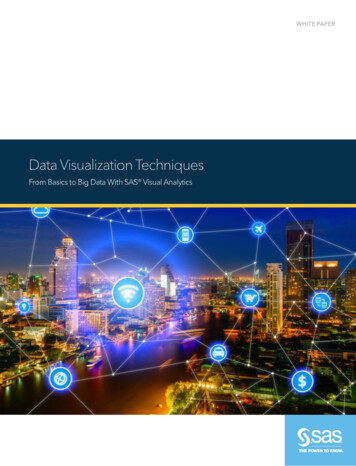
Visualizing Data with Graphs and MapsChapter 1Take a look at what the graph looks like in the Monitoring Graphs section for Atest host:So, this particular host has a bit more than one and a half gigabytes used on the rootfilesystem. But the graph is quite hard to read—it does not show how full thepartition is, relatively speaking. The y-axis starts a bit below our values and ends a bitabove them. Regarding the desired upper range limit on the y axis, we can figure outthe total disk space on the root filesystem in Monitoring Latest data:Hence, there's a total of almost 6.2 GB of space, which is also not reflected on thegraph. Let's try to make the graph slightly more readable. In the configuration of theUsed diskspace graph in the template, take a look at two options—Y axis MIN valueand Y axis MAX value. They are both set to Calculated currently, but that doesn'tseem to work too well for our current scenario. First, we want to make sure that thegraph starts at zero, so change the Y axis MIN value to Fixed. This allows us to enterany arbitrary value, but a default of zero is what we want.For the upper limit, we could calculate what 6.19 GB is in bytes and insert that value,but what if the available disk space changes? Often enough, filesystems increase either byadding physical hardware, by using Logical Volume Management (LVM), or byother means.[ 20 ]

Visualizing Data with Graphs and MapsChapter 1Does this mean we will have to update the Zabbix configuration each time this could happen?Luckily, no. There's a nice solution for situations just like this. In the Y axis MAXvalue drop-down, select Item. That adds another field and a button, so click onSelect. In the popup, click on Diskspace on / (total) in the Name column. The final yaxis configuration should look like this:If it does, click on Update. Now is the time to check out the effect on the graph—seethe Used diskspace graph in Monitoring Graphs:If the y-axis maximum is set to the amount of used diskspace, thetotal diskspace item has not received a value yet. In such a case, youcan either wait for the item to get updated or temporarily decreaseits interval.Now, the graph allows us to easily identify how full the disk is. Notice how we used agraph like this on the template. All hosts would have used total diskspace items, andthe graph would automatically scale to whatever amount of total diskspace that hosthas. This approach can also be used for used memory, or any other item where youwant to see the full scale of possible values. A potentially negative side effect couldarise when monitoring large values such as petabyte-size filesystems. With the y-axisrange spanning several petabytes, we wouldn't really see any normal changes in thedata, as a single pixel on the y-axis would be many gigabytes.[ 21 ]

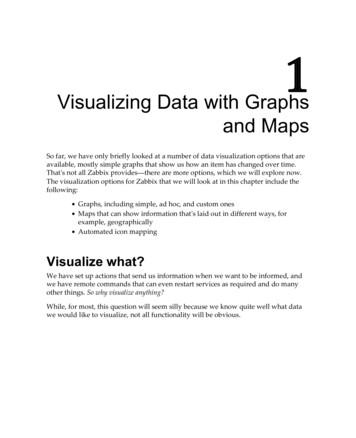
Visualizing Data with Graphs and MapsChapter 1At this time, it is not possible to set y-axis minimum and maximumseparately for left and right y-axes.Percentile lineA percentile is the threshold below which a given percentage of values fall. Forexample, if we have network traffic measurements, we could calculate that 95% ofvalues are lower than 103 Mbps, while 5% of values are higher. This allows us to filterout peaks while still having a fairly precise measurement of the bandwidth used.Actually, billing by used bandwidth most often happens by a percentile. As such, itcan be useful to plot a percentile on a network traffic graph, and luckily, Zabbix offersa way to do that. To see how this works, let's create a new graph:1. Navigate to Configuration Templates, click on Graphs next toC Template Linux, and then click on the Create graph button.2. In the Name field, enter Incoming traffic on enp0s3 withpercentile. Click on Add in the Items section and, in the popup, click onIncoming traffic on interface enp0s3 in the Name column. For this item,change the color to red. In the graph properties, mark the checkbox next toPercentile line (left) and enter 95 in that field.3. When done, click on the Add button at the bottom. Check this graph in themonitoring section:[ 22 ]

Visualizing Data with Graphs and MapsChapter 1When the percentile line is configured, it is drawn in the graph in green (although thisis different in the dark theme). Additionally, percentile information is shown in thelegend. In this example, the percentile line nicely evens out a few peaks to showaverage bandwidth usage. With 95% of the values being above the percentile line,only 5% of them are above 150 Bps.We changed the default item color from green so that the percentile line had adifferent color and it would be easier to distinguish it. Green is always used for theleft-hand side y-axis percentile line; the right-hand side y-axis percentile line wouldalways be red.We only used a single item on this graph. When there are multiple items on the sameaxis, Zabbix adds up all the values and computes the percentile based on that result.At this time, there is no way to specify the percentile for individual items in thegraph.To alert on the percentile value, the trigger function percentile() can be used. Tosto

The visualization options for Zabbix that we will look at in this chapter include the following: Graphs, including simple, ad hoc, and custom ones . graph or otherwise visually laid out information can be very helpful. We'll now look . cell for a few seconds will open a tool-tip with a color value: Visualizing Data with Graphs and Maps .