WIXLIB

Descriptive Statistics and Visualizing Datain STATABIOS 514/517R. Y. ColeyWeek of October 7, 2013

Log Files, Getting Data in STATALog files save your commandscd /home/students/rycoley/bios514-517 To change directorylog using stata-section-oct7, replace text To name log file (change stata-section-oct7) capture log close to close log fileinsheet EVdata.csv To get FEV data in

Defining, Labeling Variablestable smoke Currently coded as 1 and 2 No missing data (would be coded as 9)label define smokelabel 1 "smoker" 2 "non-smoker"label values smoke smokelabellabel define sexlabel 1 "male" 2 "female"label values sex sexlabel

Labeling Variableslabel variable age "Age (years)"label variable fev "FEV (L/s)"label variable height "Height (in)"

Descriptive StatisticsBasic commands detailed in this week’s lecture notes: summarize means centile tabstat tabulate

Descriptive Stats by Groupbysort sex: tabstat fev, stat(n mean sd min p25med p75 max) col(stat) formatbysort sex:tabulate smoke

Defining New VariablesA few ways: gen age9over age 9 gen age9over 0replace age9over 1 if age 9 gen age9over age 9 age 10 age 11. age 19

Measures of Spread Range: tabstat fev, stat(min max range) Variance: tabstat fev, stat(var) Standard Deviation: tabstat fev, stat(sd) Interquartile Range: tabstat fev, stat(p25, p75,iqr) IQR is the distance between the 25th and 75thpercentiles of the data

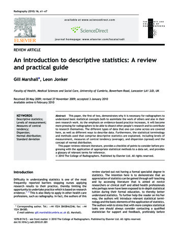
Visualizing Data- Histogramshistogram fevto save: graph export hist-fev.png, replaceHeight of each bar proportional to proportion of observationsin that bin’s range

Visualizing Data- Histogramshistogram fev, kdensity by (sex)kdensity adds smooth line estimating density

Visualizing Data- Dotplotsdotplot fevEach dot represents an observations

Visualizing Data- Box Plots a.k.a. “Box and whiskers” plots Box extends from lower quartile (25th percentile of data) toupper quartile (75th percentile) with a line at the median(50th percentile). Whiskers extend from lower quartile to “lower adjacent value”and from upper quartile to “upper adjacent value”3LAV lower quartile IQR23U AV upper quartile IQR (2 Observations outside the UAV and LAV plotted as points (Some box plots have whiskers extend to minimum andmaximum observations.)

Visualizing Data- Box Plotsgraph box fev

Visualizing Data- Box Plotsgraph box fev, over(sex)

Visualizing Data- Scatterplotsscatter fev height

Visualizing Data- Bar Chartsgen one 1graph bar (count) one, over(smoke) ytitle("frequency")

Another Examplelog using cause-of-death, text replaceset obs 10input float deaths str30 cause700142 "Heart Disease"553768 "Cancer"163538 "Cerebrovascular Disease"123013 "Chronic respiratory disease"101537 "Accidental Death"71372 "Diabetes"62034 "Flu and pneumonia"53852 "Alzheimer’s disease"39480 "Kidney disorder"32238 "Septicemia"

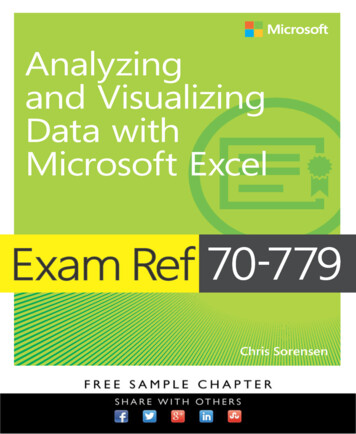
Visualizing Data- Bar Chartgen dthou deaths/1000graph hbar dthou, over(cause) ytitle("Annualdeaths (thousands)")

Visualizing Data- Bar Chartsgen dthou deaths/1000graph hbar dthou, over(cause, sort(1) descending)ytitle("Annual deaths (thousands)")

Visualizing Data- Pie Chartsgraph pie deaths, over(cause) sort descending

Visualizing Data- Pie Charts

Visualizing Data- Pie Charts

Visualizing Data- Pie Charts

Doing it all over again in R!Look at the code I have posted on the discussionboard. It is extensively commented (##)!Comments omitted here.data -read.csv("FEVdata.csv",header TRUE)names(data)dim(data)n -dim(data)[1]

(Re-)defining variablesVariables don’t have labels like in Stata. But, we can improveupon the current coding of ”smoke” and ”sex”.data SMOKE[data SMOKE 2] -0data FEMALE -data SEX 2Creating a new variable:data age9over -data AGE 9\\

Descriptive Statisticssummary(data FEV) #min, 1Q, Med, Mean, 3Q, Maxmean(data FEV)quantile(data FEV, p c(0.25, 0.5, 0.75))table(data SMOKE)xtabs( data SMOKE data FEMALE) #to get cross tabulation

Measures of Spreadrange(data FEV) #gives min and maxvar(data FEV) #variancesd(data FEV) #standard deviation

Histogramshist(data FEV, xlab "FEV (L/s)", main "Histogram of FEV")To save the graph:pdf(file "fev-hist-R.pdf")hist(data FEV, xlab "FEV (L/s)", main "Histogram of FEV")graphics.off()050Frequency100150Histogram of FEV123FEV (L/s)456

Histogramshist(data FEV, xlab "FEV (L/s)", main "Histogram of FEV",prob TRUE)lines(density(data FEV))0.20.10.0Density0.30.4Histogram of FEV123FEV (L/s)456

Histogramplot(hist(data FEV[data FEMALE 0], xlab "FEV (L/s)",main "Males", ylim c(0,80)),hist(data FEV[data FEMALE 1], xlab "FEV (L/s)",main "Females", xlim 0Males123FEV (L/s)4560123FEV (L/s)456

Boxplotboxplot(data FEV, ylab "FEV (L/s)") 5 321FEV (L/s)4

Boxplot321FEV (L/s)45boxplot(data FEV data FEMALE, ylab "FEV (L/s)",xaxt "n")axis(1, at c(1,2), labels c("Male", "Female"))MaleFemale

Scatter Plotplot(data FEV data HEIGHT, ylab "FEV (L/s)",xlab "Height (in)") 5 3 2 1FEV (L/s)4 45 505560Height (in)657075

Bar Plot0100200300400500counts -table(data SMOKE)barplot(counts, xlab "Smoker", xaxt "n")axis(1, at c(1,2), labels c("No","Yes"))NoYesSmoker

Cause of Death Example in Rn.deaths -c(700142, 553768, 163538, 123013,101537, 71372, 62034, 53852, 39480, 32238)cause -c("Heart Disease", "Cancer", "CerebrovascularDisease", "Chronic Respiratory Diesease","Accidentaldeath", "Diabetes", "Flu and Pneumonia", "Alzheimer’sDisease", "Kidney Disorder","Septicemia")n.deaths -n.deaths/1000

Cause of Death Examplepar(mar c(4,6.5,1,1))barplot(n.deaths, horiz T, yaxt "n", xlab "Number of Death(Thousands)", main "Cause of Death")text(y seq(1,11.35, 1.15), par("usr")[1], labels cause,srt 45, pos 2, xpd T, cex 0.75)conihrebrHearterCCovasRAlesFlzupiAcran heim Kicidcu atodderyPn er's neylaSentrDDDeuDptDDaieiCiabldisisisicmanea sorea seaeaemeoedeatcenitesseseseiaeahsrrCause of Death0100200300400Number of Deaths (Thousands)500600700

Cause of Death Examplepie(n.deaths, cause, main "Cause of Death" )Cause of DeathHeart DiseaseCancerSepticemiaKidney DisorderAlzheimer's DiseaseFlu and PneumoniaDiabetesAccidental deathCerebrovascular DiseaseChronic Respiratory Diesease

Visualizing Data- Histograms histogram fev to save: graph export hist-fev.png, replace Height of each bar proportional to proportion of observations in that bin’s range . Visualizing Data- Histograms histogram fev, kdensity by (sex) kdensity adds smooth line estimating density. Visualizing Data- Dotplots dotplot fev Each dot represents an observations. Visualizing Data- Box Plots a.k.a. \Box .