WIXLIB

2geoinformatics. Geoinformatics is the science that uses spatially related information andcomputational technology systems to address complex problems in the earth,environmental, geographical and related engineering disciplines with the future goal toprovide greater availability of data and tools for serving the needs of the public (Awangeand Kiema 2013). When GIS-assisted approaches are used to acquire, manage andanalyze geo-information in combination with advanced computational techniques,geoinformatics becomes a powerful tool to efficiently integrate different data andimprove the way scientific information is processed and presented (Krishna et al. 2010).The development and implementation of information and computing technology aswell as cyberinfrastructure for the earth sciences is expected to help transform the nextgeneration of interdisciplinary research. The shift to the information age (known as the“Digital Revolution”) has very significantly affected academia in which earth scientistsincreasingly rely more on digital data instead of hard copy. Hence the emergence ofevolving fields such as geoinformatics will be very important for data-intensive research,especially with the global exchange of information (i.e. the onset of “big data”).Geographic information systems are complex systems that are comprised of differentcomponents which have separate functions including data, software/hardware andpersonnel. When used collectively the components allow for broader approaches tospatial problem solving. GIS usage specializations relevant to this research includeremote sensing, programming, global navigation and positioning systems, spatial analysisand modeling, as well as other spatial science disciplines dealing with data visualizationand optimization (Wilson and Fotheringham 2008). The data management system of aGIS is typically managed via the use of integrated spatial databases that allow for the

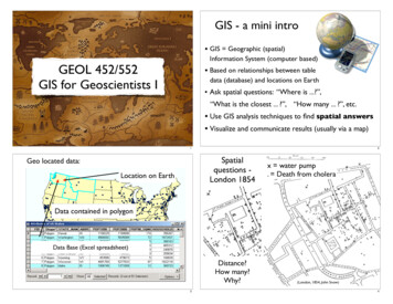
3organization of information and the determination of relationships between the data andtopology. An illustration of the database which was used as a model for the database forthis research and for optimizing field activities, and which contains information about thestudy area input data and individual oil reservoir wells, is shown in Figure 1. Additionalmore complex programs that can perform GIS geoprocessing functions (e.g.ModelBuilder) can be used to automate workflows for improving production activitiesencountered in day-to-day field work.Figure 1: Database design utilized for field services by lease operators (OCR 2014).

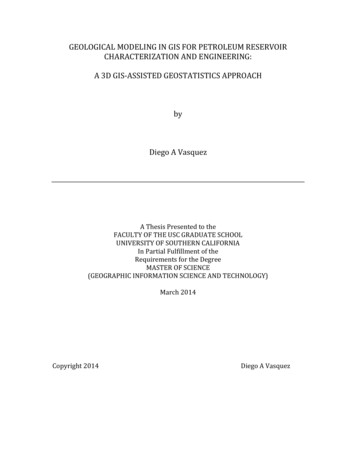
41.1.2 Thesis ObjectiveThe primary objective of this thesis project was to develop a volumetric 3D geologicalmodel of the petroleum reservoir in the study area using GIS to visualize the subsurfacedistribution of rock properties shown in Figure 2, the Abacherli reservoir within theMahala oil field of the Los Angeles Basin of Southern California.Figure 2: DEM of study area region with active geological faults (based on USGIN 2011)Interpolation of drilled well or wellbore data involves predicting values of specificvariables at unknown locations based on the measurements obtained from knownlocations using statistical principles, thereby creating a continuous surface of thesubsurface field. Earth systems are inherently complex, dynamic and contain various

5characteristics that can make reservoir characterization a very burdensome task (Caumon2010). The inclusion of geological features depends mainly on the depositionalenvironment and defines the overall geological architecture of a given reservoir (Kelkarand Perez 2002). Different geological settings may require different geostatisticalapproaches (e.g. object-based modeling or variogram-based modeling) in order toconstruct an appropriate model that honors the form of the reservoir as closely aspossible. Stationarity, defined in practice as local data averages within a spatial domainthat are approximately constant, is the most important assumption for estimation ingeostatistics. Assuming stationarity in a particular region requires that the modeldeveloped from the sampled data be applicable within the specified study area. Inreservoir analyses this assumption is necessarily subjective because of the inherentuncertainties in the subsurface and the scarcity of data which prevents researchers frombeing absolutely certain about the subsurface geology of a region in which there islimited wellbore data. In the context of this study, a region of stationarity defines thecontinuity boundaries for the study area subsurface or “field”.Geostatistics is the discipline concerned with determining the extent of that continuitywithin the region of assumed stationarity by taking advantage of the notion that valuesthat are closer to one another are more similar than values further away (i.e. as thedistance between any two values increases the similarity between the two measurementsdecreases) (Kelkar and Perez 2002). Following this assumption, geostatistical techniquesare aimed at identifying spatial relationships between variables, such as how neighboringvalues are related to each other, in order to estimate values at separate locations. Providedthat field conditions meet the criteria, one reliable approach to define this variability is

6through a statistical correlation as a function of distance, known as a variogram. In manycases where geological structures are assumed continuous throughout the reservoir, evenif a few discontinuous lithological layers act as baffles, it is appropriate to assume that thereservoir can be modeled as a whole by the use of variogram-based modeling. Figure 3illustrates a typical petroleum deposit scheme in which oil and gas are generated at thesource, migrate in direction of least resistance and are subsequently trapped andaccumulated to form petroleum reservoirs.Figure 3: Digitized hydrocarbon deposit system (based on AAPG UGM SC 2011)

71.2 Analysis Review1.2.1 Kriging ReviewKriging is a widely used conventional estimation technique that is based on alinear estimation procedure expected to provide accurate predictions of values within avolume, over an area or at an individual point within a specified field. In earth science,kriging is a favored interpolation approach compared to other methods because of itsability to include the anisotropy that rock layers of a sedimentary material exhibit ingeological formations, thus the models that are obtained via the use of kriging have moreresemblance to the true field geology (SPE PetroWiki 2013). This is in part because thelinear-weighted averaging methods used in kriging techniques depend on direction aswell as orientation, instead of only depending on distance as other interpolation methodsdo. The fundamental principle in any kriging technique is that an unknown value at anunsampled point is estimated by the product of a weighted average of neighboring values,as explained by the following simplified expression:(⃗ ) (⃗ )(Where ( ⃗ ) value at neighboring location ( ⃗ ),) weight of neighboring value and( ⃗ ) estimated value at unsampled location. The estimation procedure calculates theweights ( ) assigned to neighboring locations, which depend on the spatial relationshipbetween unsampled points and neighboring values as well as the spatial relationshipbetween neighboring points (Kelkar and Perez 2002). The relationships are obtained viathe use of a variogram model.

8Variations between the different types of variogram-based kriging methodsavailable are different depending by how the mean value is determined and used in theinterpolation (SPE PetroWiki 2013). Ordinary kriging is by far the most commonly usedkriging approach that allows for the local mean to vary and be re-estimated based onnearby (local) values thereby easing the assumption of first-order stationarity (Kelkar andPerez 2002). Ordinary kriging is better suited for this type of analysis because a truestationary global mean value for data in a reservoir is typically unknown and it cannot beassumed that the sample mean is the same as the global mean. This is due to the fact thatin any real reservoir the local mean within a neighborhood in the field can easily varyover the spatial domain.Ordinary kriging is deemed appropriate and used as the estimation technique inthis analysis. Nevertheless, it is important to consider three other types of krigingtechniques, which include simple kriging, universal kriging and cokriging. As the namesuggests simple kriging is the mathematically simplest technique where a knownstationary mean must be assumed over the entire spatial domain or study area. However,it is unrealistic to assume that we know the exact mean for all the data locations in thefield given the degree of uncertainty in the subsurface geology, therefore this techniquewas not applied in this study. The universal kriging model assumes that there is a generalpolynomial trend. However the data is not known to exhibit a trend in a particulardirection and there is no scientific justification to describe a potential trend, so universalkriging was not deemed to be more appropriate either. Cokriging is a type of krigingtechnique that uses spatial correlations from different data variable types to estimate thevalues at unsampled locations. In addition to estimating the values at unsampled locations

9with surrounding samples of the same variable type (e.g. porosity), cokriging also usesthe surrounding samples from different variables (e.g. permeability) provided theassumption that both variable types are spatially correlated to each other (Kelkar andPerez 2002). Taking advantage of the covariance between two or more spatially relatedvariables, and in theory providing a greater ability to make better predictions, cokriging isan attractive as well as commonly used approach. Nevertheless, the applicability ofcokriging to a particular field depends on if the objective is to provide a strongerprediction of a more undersampled variable relative to a more well-sampled variablegiven a strong correlation between the two variables. For example, if permeability valueswere derived from core samples for only a few wells, say 4 or 5, but electrical log valueswere obtained for all of the 13 wells and assuming spatial relationships between the coresand logs, then it would be most appropriate to “cokrige” the permeability samples withthe resistivity/spontaneous potential to provide a better permeability distribution model.But because both electrical properties in this study, spontaneous potential and resistivity(“SP” and “R”), are adequately sampled, it was decided that cokriging analysis would notbe included. Nevertheless performing cokriging between SP and R as an additionalanalysis in the future may provide useful results and information.1.2.2 Simulation ReviewAnother approach besides conventional estimation techniques such as kriging tocharacterize heterogeneous reservoirs is the use of geostatistical conditional simulationtechniques. One of the primary differences between the two is that simulation methodspreserve the variance observed in the data by relaxing some of the constraints of kriging,

10as opposed to only preserving the mean value. Conditional simulation is a type ofvariation of conventional kriging and is a stochastic modeling approach that allows forthe calculation of multiple equally probable solutions (i.e. realizations) of a regionalizedvariable by simulating the various attributes at unsampled locations, instead of estimatingthem (SPE PetroWiki 2013). A “conditional” simulation is conditioned to prior data, or inother words the hard or raw data measurements and their spatial relationships such as avariogram are honored. By providing several alternate equiprobable realizations thisapproach helps represent the true local variability thereby helping to characterize localuncertainty. This is one of the most useful properties of a simulation because all modelsare subject to uncertainty, in particular geological models because they are based onpartial sampling. This is especially true of reservoir models due to the several differentsources of uncertainty.Provided that the true value of a geological attribute is a single number but thatexact value is always unknown because of the uncertainty in the field, the practice instatistical modeling is to transform the single number into a random variable, a variate,which is a function that specifies its probability of being the true value for every likelyoutcome. The two main types of conditional simulation methods are either grid-based(a.k.a pixel-based) which operate one cell (or point) at a time, or are object-based whichoperate on groups of cells arranged within a discretized geologic shape (SPE Petrowiki2013). During each individual run the corresponding realization starts with a uniquerandom ‘navigational path’ through the discretized volume providing the order of cells(or points) to be simulated. Because the ‘path’ differs from each realization-to-realizationthe results provide differences throughout the unsampled cells which yield the local

11changes in the distribution of rock properties throughout the reservoir that are of interestfor accurate geological representations. For example, in this study running severalrealizations produced several values per variate, which then allowed for a graphicalrepresentation of the results and an approximation of the variates (Olea et al. 2012). Themethod used in this study is the grid-based approach because of the geologicalassumption that the geologic facies vary smoothly enough across the reservoir (typicaldepositional setting of shallow marine reservoirs) as opposed to sharp changes in theshape of the sedimentary body. Furthermore, there are different types of simulationmethods including annealing simulation, truncated Gaussian simulation, turning bandssimulation and sequential simulation. Sequential simulation methods are some of themost widely used in practice and are kriging-based methods where unsampled locationsare sequentially and randomly simulated until all points are included. The order and theway that locations are simulated determine the nature of the realizations. There are threetypes of sequential-simulation procedures, including Bayesian indicator, sequentialGaussian, sequential indicator. These are based on the same algorithm but with slightvariations. Sequential Gaussian Simulation (SGS) is one of the most popular, it assumesthe data follow a Gaussian distribution. Because SGS is best suited for simulatingcontinuous petrophysical variables (e.g. resistivity, spontaneous potential, porosity,permeability) it is deemed most appropriate for this study and thus was used as thesimulation method, detailed in Chapter 4.

121.2.3 Interpolation ComparisonBoth conventional estimation (kriging) and stochastic modeling (sequentialGaussian simulation) techniques are well proven, but slightly different, approaches todescribe the natural processes and attributes of geological phenomena, in this case thecharacterization of a petroleum reservoir. A useful addition is to use both of them in astudy to compare and contrast. To recap the main differences between the two: 1) krigingprovides an estimation of the mean value and its standard deviation at an individual pointgiven that the variate is represented as a random variable that follows a Gaussiandistribution, and 2) SGS selects a random deviate from the same Gaussian distributioninstead of estimating the weighted mean at each point where the simulation is selectedaccording to a uniform random number that represents the probability level (HalliburtonLandmark Software 2011). When including the simulation approach the naturalvariability of the local geology counters the blunt smoothing effects of kriging. From themultiple equiprobable realizations obtained it is possible to characterize uncertainty bycomparing a large number of realizations. Assuming the model is representative of thefield then the true value is expected to fall within the bounds of the probability.Quantification in terms of probability can be made, for example finding the mean valueof the distribution which corresponds to the highest probability. Both approachescomplement each other and are used in the analysis performed as part of this thesisresearch. The mathematical details of these methods are extensive and beyond the scopeof this report. More detailed information on the mathematical and statistical expressionscan be accessed from additional text available in the literature (e.g. McCammon 1975;Chiles and Delfiner 1999; Kelkar and Perez 2002).

131.3 Motivation1.3.1 Applicability to Petroleum Engineering and Petroleum GeologyApplied geostatistics for geological modeling and simulation is essential for successfuloil and gas production. Reservoir characterization includes determining the distribution,or the closest possible approximation, of subsurface properties of a geologic system in apetroleum field. This is essential information for improving resource management,production development and field operations (Gorell 1995). Geologic outputs obtainedfrom geostatistical models are used in a variety of important applications for petroleumand similarly for groundwater resources, including exploration, reservoir engineering andenvironmental remediation (Nobre and Sykes 1992). Having a thorough geostatisticalmodel is very important when it is used in reservoir simulators, inverse models andgeochemical models. Reliable geological models based on geostatistics can be used forspecific practices such as calculating oil production rates, remediating contaminatedaquifers, estimating the recoverable reserves (i.e. oil, gas or water), drilling newboreholes and determining hydrocarbon migration (Deutsch 2006). The combined use ofgeostatistical, simulation and inverse models enable effective reservoir engineering. Thisprovides the opportunity to predict field performance and further understand reservoirbehavior, which in turn furthers the ultimate goal of optimizing production andmaximizing hydrocarbon recovery (Coats 1969). Reservoir engineering as a subdiscipline has grown exponentially with the onset of digital technologies and computerscapable of performing larger and more complex sets of calculations. Because of this“reservoir simulation revolution” and the increasing demand for energy, geostatistical

14modeling will remain a key engineering tool in natural resource development (Stags andHerbeck 1971).The schematic diagram provided in Figure 4 illustrates the general workflow cycle ofthe “field” from a reservoir engineering perspective. First a geostatistical model(geological continuity) is developed and input into a fluid flow model (reservoirsimulator) that predicts field production, then an objective function (inverse model) isdeveloped to integrate dynamic data (field observations) and adjust the necessaryparameters (history match) until the simulations are reasonably close to the observations.The complete process assists in the validation of all model(s) included in a givenanalysis, thus providing the opportunity to achieve a validated decision-making toolensuring that optimal field performance is achieved in the future.Figure 4: Reservoir engineering results illustrating reservoir characterization/simulation scheme.

151.3.2 Importance of the Energy IndustryThe energy industry is an extremely important part of the Unites States economyand will remain a key component for economic growth in the following decades.Petroleum is currently the most important player in the energy industry and is expected tocont

interoperability across different software. Validation of the predictive geostatistical models includes performing a leave-one-out cross-validation for each borehole as well as computing a stochastic model based on the sequential Gaussian simulation algorithm, which yielded multiple realizations that were used for statistical comparison.