Transcription
Advanced Mathematical Methods in Theoretical PhysicsWintersemester 2017/2018Technische Universität BerlinPD Dr. Gernot SchallerMarch 15, 2021
iThis lecture aims at providing physics students and neighboring disciplines with a heuristictoolbox that can be used to tackle all kinds of problems. As time and resources are limited, wewill explore only small fractions of different much wider fields, and students are invited to take thelecture only as a starting point.The lecture will try to be as self-contained as possible and aims at providing rather recipes thanstrict mathematical proofs. It is not an original contribution but an excerpt of many papers, books,other lectures, and own experiences. Only a few of these have been included as references (footnotesdescribing famous scientists originate from Wikipedia and solely serve for better identification).As successful learning requires practice, the lecture (Mondays) will be accompanied by exercises. Students should turn in individual solutions to the exercises at the beginning of Wednesdayseminars (computer algebra may be used if applicable). Students may earn points for the exercisesheets, to be admitted to the final exam, they should have earned 50% of the points. After passingthe final exam, the students earn in total six ECTS credit points. To get these credit points,students therefore need to get 50 % of the exercise points and 50 % to pass the final exam.The lecture script will be made available online ns and suggestions for improvements should be addressed togernot.schaller@tu-berlin.de.The tentative content of the lecture is as follows: Integration Integral Transforms Ordinary Differential Equations Partial Differential Equations Statistics Operators
ii
Contents1 Integration of Functions1.1 Heuristic Introduction into Complex Analysis1.1.1 Differentiation over C . . . . . . . . . .1.1.2 Integration in the complex plane C . .1.1.3 Cauchy integral theorem . . . . . . . .1.1.4 Cauchy’s integral formula . . . . . . .1.1.5 Examples . . . . . . . . . . . . . . . .1.1.6 The Laurent Expansion . . . . . . . .1.1.7 The Residue Theorem . . . . . . . . .1.1.8 Principal Value integrals . . . . . . . .1.2 Useful Integration Tricks . . . . . . . . . . . .1.2.1 Standard Integrals . . . . . . . . . . .1.2.2 Integration by Differentiation . . . . .1.2.3 Saddle point approximation . . . . . .1.3 The Euler MacLaurin summation formula . .1.3.1 Bernoulli functions . . . . . . . . . . .1.3.2 The Euler-MacLaurin formula . . . . .1.3.3 Application Examples . . . . . . . . .1.4 Numerical Integration . . . . . . . . . . . . .1.4.1 The Trapezoidal Rule . . . . . . . . . .1.4.2 The Simpson Rule . . . . . . . . . . .1.4.3 Monte-Carlo integration . . . . . . . .1114567911141616171819192122242526292 Integral Transforms2.1 Fourier Transform . . . . . . . . . . . . . . . . .2.1.1 Continuous Fourier Transform . . . . . .2.1.2 Important Fourier Transforms . . . . . .2.1.3 Applications of the convolution theorem2.1.4 Discrete Fourier Transform . . . . . . . .2.2 Laplace Transform . . . . . . . . . . . . . . . .2.2.1 Definition . . . . . . . . . . . . . . . . .2.2.2 Properties . . . . . . . . . . . . . . . . .2.2.3 Applications . . . . . . . . . . . . . . . .313131333435363640433 Ordinary Differential Equations513.1 Linear ODEs with constant coefficients . . . . . . . . . . . . . . . . . . . . . . . . . 523.1.1 Properties of the Matrix Exponential . . . . . . . . . . . . . . . . . . . . . . 52iii
ivCONTENTS3.23.33.43.53.63.1.2 Numerical Computation of the matrix exponentialThe adiabatically driven Schrödinger equation . . . . . .Periodic Linear ODEs . . . . . . . . . . . . . . . . . . .Nonlinear ODEs . . . . . . . . . . . . . . . . . . . . . . .3.4.1 Separable nonlinear ODEs . . . . . . . . . . . . .3.4.2 Fixed-Point Analysis . . . . . . . . . . . . . . . .Numerical Solution . . . . . . . . . . . . . . . . . . . . .3.5.1 Runge-Kutta algorithm . . . . . . . . . . . . . . .3.5.2 Leapfrog integration . . . . . . . . . . . . . . . .3.5.3 Adaptive stepsize control . . . . . . . . . . . . . .A note on Large Systems . . . . . . . . . . . . . . . . . .4 Special Partial Differential Equations4.1 Separation Ansatz . . . . . . . . . . . . . . .4.1.1 Diffusion Equation . . . . . . . . . . .4.1.2 Damped Wave Equation . . . . . . . .4.2 Fourier Transform . . . . . . . . . . . . . . . .4.2.1 Example: Reaction-Diffusion Equation4.2.2 Example: Unbounded Wave Equation .4.2.3 Example: Fokker-Planck equation . . .4.3 Green’s functions . . . . . . . . . . . . . . . .4.3.1 Example: Poisson Equation . . . . . .4.3.2 Example: Wave Equation . . . . . . .4.4 Nonlinear Equations . . . . . . . . . . . . . .4.4.1 Example: Fisher-Kolmogorov-Equation4.4.2 Example: Korteweg-de-Vries equation .4.5 Numerical Solution: Finite Differences . . . .4.5.1 Explicit Forward-Time Discretization .4.5.2 Implicit Centered-Time discretization .4.5.3 Indexing in higher dimensions . . . . .4.5.4 Nonlinear PDEs . . . . . . . . . . . . .5 Master Equations5.1 Rate Equations . . . . . . . . . . . . . . . . . . . . .5.1.1 Example 1: Fluctuating two-level system . . .5.1.2 Example 2: Interacting quantum dots . . . . .5.2 Density Matrix Formalism . . . . . . . . . . . . . . .5.2.1 Density Matrix . . . . . . . . . . . . . . . . .5.2.2 Dynamical Evolution in a closed system . . .5.2.3 Most general evolution in an open system . .5.3 Lindblad Master Equation . . . . . . . . . . . . . . .5.3.1 Example: Master Equation for a driven cavity5.3.2 Superoperator notation . . . . . . . . . . . . .5.4 Full Counting Statistics in master equations . . . . .5.4.1 Phenomenologic Identification of Jump Terms5.4.2 Example: Single-Electron-Transistor . . . . .5.5 Entropy and Thermodynamics . . . . . . . . . . . . 111112.
CONTENTS5.5.15.5.25.5.35.5.4vSpohn’s inequality . . . . . . . . . . . .Phenomenologic definition of currents . .Thermodynamics of Lindblad equations .Nonequilibrium thermodynamics . . . .6 Canonical Operator Transformations6.1 Bogoliubov transformations . . . . . . . . . . . . . . . .6.1.1 Example: Diagonalization of a homogeneous chain6.2 Jordan-Wigner Transform . . . . . . . . . . . . . . . . .6.3 Collective Spin Models . . . . . . . . . . . . . . . . . . .6.3.1 Example: The Lipkin-Meshkov-Glick model . . .6.3.2 Holstein-Primakoff transform . . . . . . . . . . .112113114116.119. 119. 121. 121. 128. 131. 133
viCONTENTS
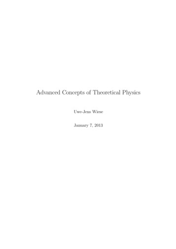
Chapter 1Integration of FunctionsIn this chapter, we first briefly review the properties of complex numbers and functions of complexnumbers. We will find that these properties can be used to solve e.g. challenging integrals in anelegant fashion.1.1Heuristic Introduction into Complex AnalysisComplex analysis treats complex-valued functions of a complex variable, i.e., maps from C toC. As will become obvious in the following, there are fundamental differences compared to realfunctions, which however can be used to simplify many relationships extremely. In the following,we will therefore for a complex-valued function f (z) always use the partitionz x iyf (z) u(x, y) iv(x, y)::{x, y R}{u, v : R2 R} ,(1.1)where x and y denote real and imaginary part of the complex variable z, and u and v the real andimaginary part of the function f (z), respectively.1.1.1Differentiation over CThe differentiability of complex-valued functions is treated in complete analogy to the real case.One fundamental difference however is that the limitf (z 0 ) f (z)z zz0 zf 0 (z) : lim0(1.2)has in the complex plane an infinite number of ways to approach z 0 z, whereas in the realcase there are just two such paths (left and right limit). In analogy to the real case we define thederivative of a complex function f (z) via the difference quotient when the limit in Eq. (1.2)a.) exists andb.) is independent of the chosen path.In this case, the function f (z) is then called in z complex differentiable. If f (z) is complexdifferentiable in a Uε -environment of z0 , it is also called holomorphic in z0 .Demanding that a function is holomorphic has strong consequences, see Fig. 1.1. It implies1
2CHAPTER 1. INTEGRATION OF FUNCTIONSiyz’ z i yFigure 1.1: For the complex-differentiable function f (x iy) u(x, y) iv(x, y) we consider thepath z 0 z once parallel to the real and onceparallel to the imaginary axis. For a complexdifferentiable function, the result must be independent of the chosen path.zz’ z xxthat the derivative can be expressed byu(x x, y) iv(x x, y) u(x, y) iv(x, y) xu(x x, y) u(x, y)v(x x, y) v(x, y) lim i lim x 0 x 0 x x u v i . x xf 0 (z) lim x 0(1.3)On the other hand one must also haveu(x, y y) iv(x, y y) u(x, y) iv(x, y) y 0i yu(x, y y) u(x, y)v(x, y y) v(x, y) lim i lim y 0 y 0i yi y u v , i y yf 0 (z) lim(1.4)since f (z) has been assumed complex differentiable. Now, comparing the real and imaginary partsof Eqns. (1.3) and (1.4) one obtains theCauchy 1 -Riemann 2 differential equations u v , x y u v , y x(1.5)which – in essence – generate the full complex analysis.The following theorem holds regarding complex differentiability:Box 1 (Complex differentiability) The function f (z) u(x, y) iv(x, y) is in z0 complexdifferentiable if and only if:1Augustin-Louis Cauchy (1789–1857) was an extremely productive french mathematician with pioneering contributions to analysis and functional calculus. He is regarded as the first modern mathematician since he strictmethodical approaches to mathematics.2Georg Friedrich Bernhard Riemann (1826–1866) was a german mathematician with numerous contributions toanalysis, differential geometry, functional calculus and number theory.
1.1. HEURISTIC INTRODUCTION INTO COMPLEX ANALYSIS31. real part u(x0 , y0 ) and imaginary part v(x0 , y0 ) are in (x0 , y0 ) totally differentiable and2. the Cauchy-Riemannschen differential equations (ux vy , uy vx ) in (x0 , y0 ) hold.Then, the derivative is given byf 0 (z0 ) ux (x0 , y0 ) ivx (x0 , y0 ) vy (x0 , y0 ) iuy (x0 , y0 ).Many functions can be analytically continued from the real case to the full complex plane C: the sine function (holomorphic in the full complex plane)sin(z) X( 1)n z 2n 1(1.6)(2n 1)!n 0 the cosine function (holomorphic in the full complex plane)cos(z) X( 1)n z 2n(1.7)(2n)!n 0 the exponential function (holomorphic in C)exp(z) cos(z) i sin(z) Xznn!n 0 Xn 0,(iz)2n(iz)2n 1 (2n)!(2n 1)!(1.8) exp(iz)The last relation reduces for z R to the well-known Euler 3 - Moivre4(1.9)formula.We would like to summarize a few properties of the complex derivative:1. Since the definition is analogous to the real derivative we also have in the complex plane Cthe product rule, quotient rule, and the chain rule.2. Real- and Imaginary part of holomorphic functions obey the Laplace 5 equation: uxx uyy 0 vxx vyy . This is a direct consequence of the Cauchy-Riemann differential equations (1.5).This also implies that when a holomorphic function is known at the boundary of an areaG C, it is fixed for all x G.3. It is easy to show that all polynomials in z are in C holomorphic.4. There are fundamental differences to R2 . For example, the function f (z) z z x2 y 2is totally differentiable in R2 but not holomorphic, since the Cauchy-Riemann differentialequations (1.5) are not obeyed.3Leonhard Euler (1707–1783) was a swiss mathematician with important contributions to analysis. His sonJohann Albrecht Euler also became a mathematician but contributed also to astronomy.4Abraham de Moivre (1667–1754) was a french mathematician most notably known for the formulan[cos(z) i sin(z)] cos(nz) i sin(nz).5Pierre-Simon (Marquis de) Laplace (1749–1827) was a french mathematician, physicist and astronomer. Hecontributed greatly to astronomy and physics, which forced him to developed new mathematical tools, which arestill important today.
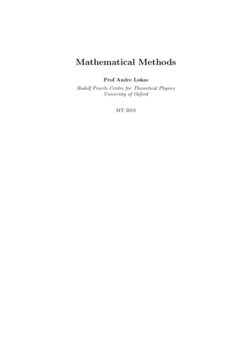
4CHAPTER 1. INTEGRATION OF FUNCTIONSz2iyc(t)Figure 1.2: In contrast to the real numbers a pathbetween points z1 and z2 in the complex planemust be specified to fix the integral. This can beconveniently done by choosing a parametrizationof a contour c(t) x(t) iy(t) with parameter t.1.1.2z1xIntegration in the complex plane CAs was already the case with differentiation, also for the integration a path must be fixed – instark contrast to the real case, see Fig. 1.2. As in the real case the integral along a contour isdefined via the Riemann sum. For its practical calculation however one uses a parametrization ofthe integration contour c by a curve c(t) : [α, β] R c C in the following way:Z βZf [c(t)]ċ(t)dt .(1.10)f (z)dz αcThis maps complex integrals to real ones.Fundamental example of complex calculusWe consider the closed integral in counterclockwise (mathematical) rotation along a circle withradius R and center z0 over the function f (z) (z z0 )n : n Z. The parametrization of thecontour is given by z(t) z0 Reit : t 0 . . . 2π. This impliesZ 2πInRn 1 ei(n 1)t dt(z z0 ) dz i0SR (z0 )Rn 1n 1ei(n 1)t2πi 2πi0: n 1:else In(z z0 ) dz SR (z0 )2π0 : n 6 1: n 1(n Z) .(1.11)For n 6 1 the vanishing of the integral follows from the periodicity of the exponential function (1.8). For n 1 the function is just constant along the contour, such that the value of theintegral is given by the length of the path. Many theorems of complex calculus may be tracedback to this fundamental example.In the complex plane the integral has similiar properties as in the real case:1. Since contour integrals are mapped to real integrals via parametrizations of the path it followsthat the integral is linear.2. For the same reason, the sign of an integral changes when the contour is traversed in theopposite direction (e.g. clockwise in the fundamental example).R3. The analogy to path integrals in R3 (for example regarding the work W c F d r ) leads tothe valid question:When are complex integrals independent of the chosen path?
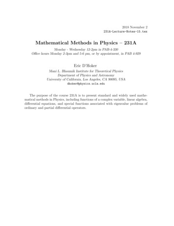
1.1. HEURISTIC INTRODUCTION INTO COMPLEX ANALYSIS1.1.35Cauchy integral theoremBox 2 (Cauchy’s integral theorem) Let G C be a bounded and simply connected (no holes)area. Let f in G be holomorphic and let c be a closed curve that is fully contained in G. Then onehas:If (z)dz 0 .(1.12)cA vanishing integral over a closed curve does of course also imply that the integral between twopoints is independent on the path (simply form a closed curve by adding two baths between twopoints). Here, we would just like to sketch the proof of Cauchy’s theorem. First we separate realand imaginary parts:IIIf (z)dz [u(x, y)dx v(x, y)dy] i [u(x, y)dy v(x, y)dx] .(1.13)cccTo both integrals we can apply the two-dimensional Stokes theorem ZZ II Fy Fx [Fx (x, y)dx Fy (x, y)dy] dxdy .F d r x yA A A(1.14)When we do now in Eq. (1.13) identify in the first integral Fx u(x, y), Fy v(x, y) and in thesecond integral Fx v(x, y), Fy u(x, y) we obtain ZZZZI v u u vdxdy dxdyf (z)dz i .(1.15) x y x yA(c)A(c)cThe terms in round brackets vanish for holomorphic functions f (z), since they constitute nothingbut the Cauchy-Riemann differential equations (1.5).Cauchy’s integral theorem is useful for the calculation of many contour integrals. Consider,for example, the function f (z) (z z0 ) 1 . It is holomorphic for all z 6 at z z0 aH z0 but has 1pole. When now z0 is not enclosed by the integration contour c, one has c (z z0 ) dz 0. If, incontrast, z0 is inside the contour specified by c, the pole can be cut out by a modified integrationpath c0 (as depicted in Fig. 1.3) to render f holomorphic in the area surrounded by c0 . Then, thearea enclosed by the modified curve c0 c c1 S̄ε (z0 ) c2 does no longer contain a pole of f .Furthermore, for a closed path c and a closed circle S̄ε (z0 ) the integrals over c1 and c2 mutuallycancel as f (z) is continuous and these paths are traversed with opposite direction. Since thecircle S̄ε (z0 ) is traversed with negative (clockwise) orientation, one obtains – with the fundamentalexample (1.11) – for the complete integralIZZZf (z)dz f (z)dz 2πi .(1.16)f (z)dz 0 f (z)dz c0cS̄ε (z0 )This implies for arbitrary integration contours c: I0 1(z z0 ) dz 2πicc: z0 /c,: z0 c(1.17)i.e., whereas the fundamental example was only valid for a circular contours, the above result ismuch more general.
6CHAPTER 1. INTEGRATION OF FUNCTIONSc2z0c1cS ε(z0 )Figure 1.3: Appropriate excision of a singularityat z z0 . The modified curve c0 c c1 S̄ε (z0 ) c2 does no longer enclose a singularity.In addition, it is directly obvious that the contributions c1 and c2 cancel each other since the aretraversed at oppositeorientation.Therefore, oneHHactually has c f (z)dz S̄ε (z0 ) f (z)dz 0.1.1.4Cauchy’s integral formulaBox 3 (Cauchy’s integral formula) Let G C be bounded and f in G be holomorphic andcontinous at the boundary G. Let G be bounded by a finite number of disjoint curves ci . Thenone has: If (z)2πif (z0 ) : z0 Gdz .(1.18)0: z0 /G G z z0Also here we would like to provide a sketch for the proof: Since the case z0 / G can be mapped toCauchy’s integral theorem we will only consider the interesting case z0 G. Then, the integrandhas a pole at z z0 , which – compare Fig. 1.3 – is excised by a small circle from G. In analogy tothe previous example one obtains following Cauchy’s integral theoremI GZ 0f (z0 εeiϕ ) iϕf (z)dz limiεe dϕε 0 2πz z0εeiϕZ 2π ilim f (z0 εeiϕ )dϕε 0Z0 2π if (z0 )dϕ 2πif (z0 ) .(1.19)0A first observation regarding Eq. (1.18) is that all values of the function f (z) in G are completelydetermined by its values at the boundary. This is a consequence of the Cauchy-Riemann differentialequations as these imply that f (x, y) is a solution to the Laplace equation (which is completelydetermined by given boundary conditions [f ( G)]). Therefore, Eq. (1.18) can be regarded a usefulmethod to solve two-dimensional boundary problems on Laplace’s equation.Eq. (1.18) can be easily generalized to poles of higher order. Particularly interesting is ofcourse only the case z0 G. By performing multiple derivatives z 0 on both sides of Eq. (1.18)
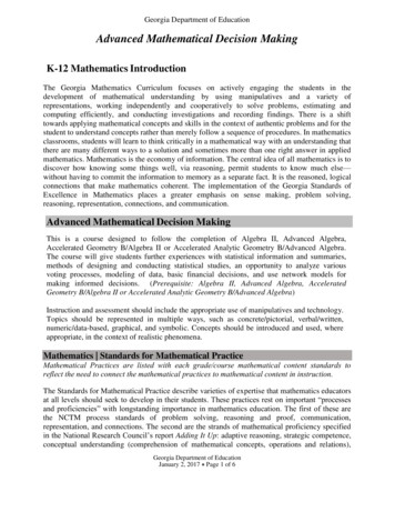
1.1. HEURISTIC INTRODUCTION INTO COMPLEX ANALYSIS7one obtainsIf (z)dz ,2 G (z z0 )If (z)002πif (z0 ) 1 · 2 ·dz ,3 G (z z0 )If (z)000dz2πif (z0 ) 1 · 2 · 3 ·4 G (z z0 )02πif (z0 ) 1 ·.For the n-th derivative one obtains Cauchy’s general integral formula:If (z)2πi (n)f (z0 )(n 0, 1, 2, . . .) ,dz n 1n! G (z z0 )(1.20)(1.21)which holds of course only for z0 G. With this formula also integrals around higher-order polescan be calculated.1.1.5ExamplesCauchy’s integral theorem and Cauchy’s integral formula are often used to calculate real-valuedintegrals – these just have to be suitably continued into the complex plane. In the following, wewill demonstrate this analytic continuation with some examples.1. The integralZ I dx 1x2withf (x) x21 1(1.22)has the solution π, since the antiderivative of f (x) is arctan. However, also without knowingthis one can find the solution directly with Eq. (1.18). The analytic continuation of f (x) tothe full complex plane is given byf (z) z211 . 1(z i)(z i)(1.23)Obviously, there exist two poles at z i. When we supplement the integral along the realaxis with the semicircle in the upper complex half-plane as depicted in Fig. 1.4, we see thatonly one pole (z i) resides inside the integration contour. In the limit limR howeverthe upper semicircle does not contribute, since f (z) decays in the far-field as R 2 , whereasthe length of the semicircle only grows linearly in R. This impliesZ IdxF (z)1I dzwithF (z) 2z i x 1c z i2πi 2πiF (i) π.(1.24)2i2. When we consider the integral over the parametrization of a conic section, i.e., over an ellipseZ 2πZ 2πdϕdϕI :0 ε 1(1.25)ε1 ε cos ϕ1 2 (eiϕ e iϕ )00
8CHAPTER 1. INTEGRATION OF FUNCTIONSyFigure 1.4: Closure of a complex integral in theupper complex half-plane. It is essential to verify that the integrand vanishes in the upper arcof radius R faster than 1/R as R , sinceotherwise its contribution cannot be neglected.i RR ixwe can use the substitution z(ϕ) eiϕ to map the integral to a closed integral along the unitcircle around the originII21dzdz I εz12i S1 (0) z 2 z zεi S1 (0) z 2ε z 1I2dz ,(1.26)εi S1 (0) (z z1 )(z z2 )r11wherez1 1:inside S1 (0)εε2r11z2 1:outside S1 (0)(1.27)εε2With Eq. (1.18) it follows thatI 122π12πq2πi .εiz1 z2ε11 ε22 1(1.28)ε3. The integralZ I 0dx1 (x2 a2 )22Z dx1 (x2 a2 )22Z dz: a 0(z ia)2 (z ia)2(1.29)can as before be closed by a semicircle in the complex plane, see Fig. 1.5. Here, the integrandvanishes even faster than in our first example, such that the contribution of the uppersemicircle need not be considered for the same reasons. However, here we have a secondorder pole residing at z ia, such that Cauchy’s general integral formula should be usedI11dz11 dI lim 2πi222 R c (z ia) (z ia)21! dz (z ia)2 z ia 2πiπ 3.(1.30) 3(z ia) z ia 4aWe note that the result is an odd function of a, whereas the true solution to the integralmust be an even function of a. This can be resolved by the fact that if a were negative,we could e.g. consider the same residue by closing the contour in the lower complex plane.Eventually, this would include a different orientation and thereby lead to a negative sign.
1.1. HEURISTIC INTRODUCTION INTO COMPLEX ANALYSIS9yia RR iaxFigure 1.5: Closure of a contour in the uppercomplex plane. We have implicitly assumed herethat a 0.4. Using the same contour as before we can also solve the integral (assuming k 0)Z ikzZ Z e dzeikz dzcos(kx)dx ,I 2222 z a (z ia)(z ia) x a(1.31)which e.g. shows up in the calculation of many Fourier 6 transforms. Above, we havealready used that the integral over the imaginary part vanishes due to symmetry arguments(odd function). Here, we have just as in Fig. 1.5 two poles, but of first order at z ia.Furthermore, in contrast to the previous cases we have to be cautious: The contour should beclosed in the upper half-plane, since in the lower half-plane (y 0) the exponential function(exp(ikz) exp(ikx) exp( ky)) would not be bounded. When we would close in the lowerhalf-plane, the contribution from the semi-circle would therefore not vanish. Closing thereforein the upper half-plane, we obtainI 2πieikzz ia z iaπ kae.a(1.32)For k 0 we would have to choose the opposite contour, but the symmetry of the cosfunction suggests that the result must be the same and we simply have to replace k k inthe result.1.1.6The Laurent ExpansionBox 4 (Laurent Expansion) Let f (z) be holomorphic inside the annulus (doughnut)K(z0 , r, R) {z C : 0 r z z0 R }. Then define for all ρ with r ρ RI1f (z)ak dz k Z(1.33)2πi Sρ (z0 ) (z z0 )k 1Then one has:a. The ak do not depend on ρ and6Jean Baptiste Joseph Fourier (1768–1830) was a french mathematician and physicist. He was interested in heatconductance properties of solids (Fourier’s law) and his Fourier analysis is a basis of modern physics and technology.
10CHAPTER 1. INTEGRATION OF FUNCTIONSb. for all z K(z0 , r, R) it follows that f is given byf (z) Xan (z z0 )n .(1.34)n The above expansion is also called Laurent 7 -Expansion. In contrast to the conventional Taylor8expansion we also observe terms with poles (ak with k 0). From the definition of the coefficientsabove it furthermore follows that the Laurent-expansion is unique.This in turn implies that in case f (z) can at z z0 be expanded into a Taylor-Series, then thisTaylor series is also the Laurent-series. In this case it just happens that many coefficients vanishak 0 0.Here, we just want to show that the calculation of the expansion coefficients ak is self-consistent.For this we insert the expansion (1.34) in Eq. (1.33)II (z z0 )l1 X1 Xaldz al(z z0 )l k 1 dz .ak k 12πi l 2πi l Sρ (z0 ) (z z0 )Sρ (z0 )(1.35)Using the fundamental example of complex calculus from Eq. (1.11) it follows that all terms exceptone (for l k 1 1, i.e., for l k) in the sum vanish. This leads to X1al δkl ak .ak 2πi2πil (1.36)This shows that the definition of the expansion coefficients is self-consistent.The Laurent-expansion is often used to classify isolated singularities. Isolated singularitieshave in their Uε -environment no further singularity – a typical counter-example is the functionf (z) z, which is non-holomorphic on the complete negative real axis (where it has no isolatedsingularities).To summarize, it is said that f (z) has at z z0 a curable singularity, when the limit limz z0 : f (z0 ) exists and is independent on theapproaching path. In the Laurent series all coefficients ak 0 vanish in this case. A popularexample for this situation is sin(z)/z, which has a curable singularity at z 0. pole of order m, when in the Laurent series of f (z) around z0 the first non-vanishingcoefficient is a m , i.e., when a m 6 0 , ak m 0. For example, the function f (z) 1/(z i)3has a third order pole at z i. essential singularity, when in the Laurent series expansion of f (z) there is no first nonvanishing coefficient, as is e.g. the case for f (z) exp(1/z) at z 0.7Pierre Alphonse Laurent (1813–1854) was a french mathematician working as an engineer in the french army.His only known contribution – the investigation of the convergence properties of the Laurent series expansion – waspublished post mortem.8Brook Taylor (1685–1731) was a british mathematician. He found his expansion already in 1712 but its importance for differential calculus was noted much later.
1.1. HEURISTIC INTRODUCTION INTO COMPLEX ANALYSIS1.1.711The Residue TheoremBox 5 (Residue) Let the Laurent expansion of a function f (z) be known around z0 . Then, theexpansion coefficient a 1 is called the residue of f at z0 , i.e.,I1Resf (z) a 1 f (z)dz .(1.37)z z02πi Sρ (z0 )Obviously, we have for the fundamental example with f (z) (z z0 ) 1 for the residue Resf (z) 1.z z0Furthermore, the integral theorem by Cauchy also implies that the residue vanishes at places wheref (z) is holomorphic. The residue theorem combines all theorems stated before and is one of themost important tools in mathemetics.Box 6 (Residue Theorem) Let G C be an area bounded by a finite number of piecewisecontinuous curves. Let furthermore f be at the boundary G and also inside G holomorphic – upto a finite number of isolated singularities {z1 , z2 , . . . , zn 1 , zn } that are all in G. Then one has:If (z)dz 2πi GnXk 1Res f (z) .(1.38)z zkHere we would also like to provide a sketch of the proof. We will need the Laurent expansion andCauchy’s integral theorem. To obtain an area within which the function is completely holomorphicwe excise the singularities as demonstrated in Fig. 1.6.The ρk have to be chosen such that the Laurent-expansion of f around zk converges on thecircle described by Sρk (zk ). Now we insert at each singularity for f (z) the Laurent expansionP (k)around the respective singularity f (z) l al (z zk )lIf (z)dz Gn X X(k)alk 1 l nX 2πiIl(z zk ) dz Sρk (zk )n X X(k)al 2πiδl, 1k 1 l Res f (z) ,k 1z zk(1.39)where we have used the fundamental example of complex calculus (1.11).Therefore, the residue theorem allows one do calculate path integrals that enclose multiplesingularities. Very often, poles show up in these integrals, and the formula for the calculation ofresidues in Eq. (1.37) is rather unpractical for this purpose, since it requires the parametrizationof an integral. Therefore, we would like to discuss a procedure that allows the efficient calculationof residues at poles of nth order.Let f (z) have at z z0 a pole of order m. Then, f (z) can be represented asf (z) a ma 2a 1 . a0 . . . .m2(z z0 )(z z0 )(z z0 )(1.40)
12CHAPTER 1. INTEGRATION OF FUNCTIONSz1z2z4Figure 1.6: The singularities in G can beexcisedH with circles ofPradiiH ρk , which implies G f (z)dz nk 1 S̄ρ (zk ) f (z)dz kP H nk 1 Sρ (zk ) f (z)dz. Here, S̄ρk (zk ) denote thekclockwise orientation as depicted and Sρk (zk )the positive orientation (cou
Advanced Mathematical Methods in Theoretical Physics Wintersemester 2017/2018 Technische Universit at Berlin PD Dr. Gernot Schaller March 15, 2021. i This lecture aims at providing physics students and neighboring disciplines with a heuristic toolbox that can be used to tackle all kinds of problems. As time and resources are limited, we