WIXLIB

ematical models and mathematical statistics/econometric methods.The study of economic social issues cannot simply involve real world in its experiment,so it not only requires theoretical analysis based on inherent logical inference and, moreoften than not, vertical and horizontal comparisons from the larger perspective of historyso as to draw experience and lessons, but also needs tools of statistics and econometrics todo empirical quantitative analysis or test, the three of which are all indispensable. Whenconducting economic analysis or giving policy suggestions in the realm of modern economics, the theoretical analysis often combines theory, history, and statistics, presentingnot only theoretical analysis of inherent logic and comparative analysis from the historicalperspective but also empirical and quantitative analysis with statistical tools for examination and investigation. Indeed, in the final analysis, all knowledge is history, all scienceis logics, and all judgment is statistics.As such, it is not surprising that mathematics and mathematical statistics/econometricsare used as the basic analytical tools, and also become the most important analytical toolsin every field of economics. For those who study economics and conduct research, it isnecessary to grasp enough knowledge of mathematics and mathematical statistics. Therefore, it is of great necessity to master sufficient mathematical knowledge if you want tolearn economics well, conduct economic research and become a good economist.1.2Advantages of Mathematical ApproachMathematical approach has the following advantages:(1) It makes the language more precise and the statement of assumptionsmore clear, which can deduce many unnecessary debates resulting frominaccurate definitions.(2) It makes the analytical logic more rigorous and clearly states the boundary,application scope and conditions for a conclusion to hold. Otherwise, theabuse of a theory may occur.(3) Mathematics can help obtain the results that cannot be easily attainedthrough intuition.(4) It helps improve and extend the existing economic theories.2

It is, however, noteworthy a good master of mathematics cannot guarantee to bea good economist. It also requires fully understanding the analytical framework andresearch methodologies of economics, and having a good intuition and insight of realeconomic environments and economic issues. The study of economics not only calls for theunderstanding of some terms, concepts and results from the perspective of mathematics(including geometry), but more importantly, even when those are given by mathematicallanguage or geometric figure, we need to get to their economic meaning and the underlyingprofound economic thoughts and ideals. Thus we should avoid being confused by themathematical formulas or symbols in the study of economics.All in all, to become a good economist, you need to be of original, creative andacademic way of thinking.3

Chapter 2Economic Models2.1Ingredients of a Mathematical ModelA economic model is merely a theoretical framework, and there is no inherent reason whyit must mathematical. If the model is mathematical, however, it will usually consist of aset of equations designed to describe the structure of the model. By relating a numberof variables to one another in certain ways, these equations give mathematical form tothe set of analytical assumptions adopted. Then, through application of the relevantmathematical operations to these equations, we may seek to derive a set of conclusionswhich logically follow from those assumptions.2.2The Real-Number SystemWhole numbers such as 1, 2, · · · are called positive numbers; these are the numbers mostfrequently used in counting. Their negative counterparts 1, 2, 3, · · · are called negative integers. The number 0 (zero), on the other hand, is neither positive nor negative,and it is in that sense unique. Let us lump all the positive and negative integers and thenumber zero into a single category, referring to them collectively as the set of all integers.Integers of course, do not exhaust all the possible numbers, for we have fractions, suchas 23 ,5,4and 73 ,, which – if placed on a ruler – would fall between the integers. Also,we have negative fractions, such as 12 and 25 . Together, these make up the set of allfractions.4

The common property of all fractional number is that each is expressible as a ratioof two integers; thus fractions qualify for the designation rational numbers (in this usage,rational means ratio-nal). But integers are also rational, because any integer n can beconsidered as the ratio n/1. The set of all fractions together with the set of all integersfrom the set of all rational numbers.Once the notion of rational numbers is used, however, there naturally arises the conceptof irrational numbers – numbers that cannot be expressed as raios of a pair of integers. One example is 2 1.4142 · · · . Another is π 3.1415 · · · .Each irrational number, if placed on a ruler, would fall between two rational numbers,so that, just as the fraction fill in the gaps between the integers on a ruler, the irrationalnumber fill in the gaps between rational numbers. The result of this filling-in processis a continuum of numbers, all of which are so-called “real numbers.” This continuumconstitutes the set of all real numbers, which is often denoted by the symbol R.2.3The Concept of SetsA set is simply a collection of distinct objects. The objects may be a group of distinctnumbers, or something else. Thus, all students enrolled in a particular economics coursecan be considered a set, just as the three integers 2, 3, and 4 can form a set. The objectin a set are called the elements of the set.There are two alternative ways of writing a set: by enumeration and by description.If we let S represent the set of three numbers 2, 3 and 4, we write by enumeration of theelements, S {2, 3, 4}. But if we let I denote the set of all positive integers, enumerationbecomes difficult, and we may instead describe the elements and write I {x x is apositive integer}, which is read as follows: “I is the set of all x such that x is a positiveinteger.” Note that the braces are used enclose the set in both cases. In the descriptiveapproach, a vertical bar or a colon is always inserted to separate the general symbol forthe elements from the description of the elements.A set with finite number of elements is called a finite set. Set I with an infinitenumber of elements is an example of an infinite set. Finite sets are always denumerable(or countable), i.e., their elements can be counted one by one in the sequence 1, 2, 3, · · · .5

Infinite sets may, however, be either denumerable (set I above) or nondenumerable (forexample, J {x 2 x 5}).Membership in a set is indicated by the symbol (a variant of the Greek letter epsilonϵ for “element”), which is read: “is an element of.”If two sets S1 and S2 happen to contain identical elements,S1 {1, 2, a, b} and S2 {2, b, 1, a}then S1 and S2 are said to be equal (S1 S2 ). Note that the order of appearance of theelements in a set is immaterial.If we have two sets T {1, 2, 5, 7, 9} and S {2, 5, 9}, then S is subset of T , becauseeach element of S is also an element of T . A more formal statement of this is: S is subsetof T if and only if x S implies x T . We write S T or T S.It is possible that two sets happen to be subsets of each other. When this occurs,however, we can be sure that these two sets are equal.If a set have n elements, a total of 2n subsets can be formed from those elements. Forexample, the subsets of {1, 2} are: , {1}, {2} and {1, 2}.If two sets have no elements in common at all, the two sets are said to be disjoint.The union of two sets A and B is a new set containing elements belong to A, or to B,or to both A and B. The union set is symbolized by A B (read: “A union B”).Example 2.3.1 If A {1, 2, 3}, B {2, 3, 4, 5}, then A B {1, 2, 3, 4, 5}.The intersection of two sets A and B, on the other hand, is a new set which containsthose elements (and only those elements) belonging to both A and B. The intersectionset is symbolized by A B (read: “A intersection B”).Example 2.3.2 If A {1, 2, 3}, A {4, 5, 6}, then A B .In a particular context of discussion, if the only numbers used are the set of the firstseven positive integers, we may refer to it as the universal set U . Then, with a given set,say A {3, 6, 7}, we can define another set Ā (read: “the complement of A”) as the setthat contains all the numbers in the universal set U which are not in the set A. That is:Ā {1, 2, 4, 5}.Example 2.3.3 If U {5, 6, 7, 8, 9}, A {6, 5}, then Ā {7, 8, 9}.6

Properties of unions and intersections:A (B C) (A B) CA (B C) (A B) CA (B C) (A B) (A C)A (B C) (A B) (A C)2.4Relations and FunctionsAn ordered pair (a, b) is a pair of mathematical objects. The order in which the objectsappear in the pair is significant: the ordered pair (a, b) is different from the ordered pair(b, a) unless a b. In contrast, a set of two elements is an unordered pair : the unorderedpair {a, b} equals the unordered pair {b, a}. Similar concepts apply to a set with morethan two elements, ordered triples, quadruples, quintuples, etc., are called ordered sets.Example 2.4.1 To show the age and weight of each student in a class, we can formordered pairs (a, w), in which the first element indicates the age (in years) and the secondelement indicates the weight (in pounds). Then (19, 128) and (128, 19) would obviouslymean different things.Suppose, from two given sets, x {1, 2} and y {3, 4}, we wish to form all thepossible ordered pairs with the first element taken from set x and the second elementtaken from set y. The result will be the set of four ordered pairs (1,2), (1,4), (2,3), and(2,4). This set is called the Cartesian product, or direct product, of the sets x and y andis denoted by x y (read “x cross y”).Extending this idea, we may also define the Cartesian product of three sets x, y, andz as follows:x y z {(a, b, c) a x, b y, c z}which is the set of ordered triples.Example 2.4.2 If the sets x, y, and z each consist of all the real numbers, the Cartesianproduct will correspond to the set of all points in a three-dimension space. This may bedenoted by R R R, or more simply, R3 .7

Example 2.4.3 The set {(x, y) y 2x} is a set of ordered pairs including, for example,(1,2), (0,0), and (-1,-2). It constitutes a relation, and its graphical counterpart is the setof points lying on the straight line y 2x.Example 2.4.4 The set {(x, y) y x} is a set of ordered pairs including, for example,(1,0), (0,0), (1,1), and (1,-4). The set corresponds the set of all points lying on below thestraight line y x.As a special case, however, a relation may be such that for each x value there existsonly one corresponding y value. The relation in example 2.4.3 is a case in point. In thatcase, y is said to be a function of x, and this is denoted by y f (x), which is read: “yequals f of x.” A function is therefore a set of ordered pairs with the property that any xvalue uniquely determines a y value. It should be clear that a function must be a relation,but a relation may not be a function.A function is also called a mapping, or transformation; both words denote the actionof associating one thing with another. In the statement y f (x), the functional notationf may thus be interpreted to mean a rule by which the set x is “mapped” (“transformed”)into the set y. Thus we may writef :x ywhere the arrow indicates mapping, and the letter f symbolically specifies a rule of mapping.In the function y f (x), x is referred to as the argument of the function, and y iscalled the value of the function. We shall also alternatively refer to x as the independentvariable and y as the dependent variable. The set of all permissible values that x can takein a given context is known as the domain of the function, which may be a subset of theset of all real numbers. The y value into which an x value is mapped is called the imageof that x value. The set of all images is called the range of the function, which is the setof all values that the y variable will take. Thus the domain pertains to the independentvariable x, and the range has to do with the dependent variable y.2.5Types of FunctionA function whose range consists of only one element is called a constant function.8

Example 2.5.1 The function y f (x) 7 is a constant function.The constant function is actually a “degenerated” case of what are known as polynomial functions. A polynomial functions of a single variable has the general formy a0 a1 x a2 x2 · · · an xnin which each term contains a coefficient as well as a nonnegative-integer power of thevariable x.Depending on the value of the integer n (which specifies the highest power of x), wehave several subclasses of polynomial function:Case of n 0 : y a0[constant function]Case of n 1 : y a0 a1 x[linear function]Case of n 2 : y a0 a1 x a2 x2[quadritic function]Case of n 3 : y a0 a1 x a2 x2 a3 x3 [ cubic function]A function such asy x2x 1 2x 4in which y is expressed as a ratio of two polynomials in the variable x, is known as arational function (again, meaning ratio-nal ). According to the definition, any polynomialfunction must itself be a rational function, because it can always be expressed as a ratioto 1, which is a constant function.Any function expressed in terms of polynomials and or roots (such as square root) ofpolynomials is an algebraic function. Accordingly, the function discussed thus far are all algebraic. A function such as y x2 1 is not rational, yet it is algebraic.However, exponential functions such as y bx , in which the independent variableappears in the exponent, are nonalgebraic. The closely related logarithmic functions, suchas y logb x, are also nonalgebraic.Rules of Exponents:Rule 1: xm xn xm nxm xm n (x ̸ 0)nx1Rule 3: x n nxRule 2:9

Rule 4: x0 1 (x ̸ 0) 1Rule 5: x n n xRule 6: (xm )n xmnRule 7: xm y m (xy)m2.6Functions of Two or More Independent VariablesThus for far, we have considered only functions of a single independent variable, y f (x). But the concept of a function can be readily extended to the case of two or moreindependent variables. Given a functionz g(x, y)a given pair of x and y values will uniquely determine a value of the dependent variablez. Such a function is exemplified byz ax by or z a0 a1 x a2 x2 b1 y b2 y 2Functions of more than one variables can be classified into various types, too. Forinstance, a function of the formy a1 x1 a2 x2 · · · an xnis a linear function, whose characteristic is that every variable is raised to the first poweronly. A quadratic function, on the other hand, involves first and second powers of one ormore independent variables, but the sum of exponents of the variables appearing in anysingle term must not exceed two.Example 2.6.1 y ax2 bxy cy 2 dx ey f is a quadratic function.2.7Levels of GeneralityIn discussing the various types of function, we have without explicit notice introducingexamples of functions that pertain to varying levels of generality. In certain instances, wehave written functions in the formy 7, y 6x 4, y x2 3x 1 (etc.)10

Not only are these expressed in terms of numerical coefficients, but they also indicatespecifically whether each function is constant, linear, or quadratic. In terms of graphs,each such function will give rise to a well-defined unique curve. In view of the numericalnature of these functions, the solutions of the model based on them will emerge as numerical values also. The drawback is that, if we wish to know how our analytical conclusionwill change when a different set of numerical coefficients comes into effect, we must gothrough the reasoning process afresh each time. Thus, the result obtained from specificfunctions have very little generality.On a more general level of discussion and analysis, there are functions in the formy a, y bx a, y cx2 bx a (etc.)Since parameters are used, each function represents not a single curve but a whole familyof curves. With parametric functions, the outcome of mathematical operations will alsobe in terms of parameters. These results are more general.In order to attain an even higher level of generality, we may resort to the generalfunction statement y f (x), or z g(x, y). When expressed in this form, the functionsis not restricted to being either linear, quadratic, exponential, or trigonometric – all ofwhich are subsumed under the notation. The analytical result based on such a generalformulation will therefore have the most general applicability.11

Chapter 3Equilibrium Analysis in Economics3.1The Meaning of EquilibriumLike any economic term, equilibrium can be defined in various ways. One definition hereis that an equilibrium for a specific model is a situation that is characterized by a lackof tendency to change. Or more generally, it means that from the various feasible andavailable choices, choose “best” one according to a certain criterion, and the one beingfinally chosen is called an equilibrium. It is for this reason that the analysis of equilibriumis referred to as statics. The fact that an equilibrium implies no tendency to change maytempt one to conclude that an equilibrium necessarily constitutes a desirable or ideal stateof affairs.This chapter provides two examples of equilibrium. One is the equilibrium attained bya market model under given demand and supply conditions. The other is the equilibriumof national income model under given conditions of consumption and investment patterns.We will use these two models as running examples throughout the course.3.2Partial Market Equilibrium - A Linear ModelIn a static-equilibrium model, the standard problem is that of finding the set of values ofthe endogenous variables which will satisfy the equilibrium conditions of model.12

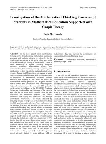
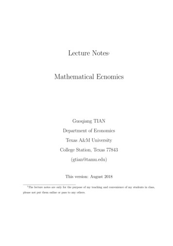
Partial-Equilibrium Market ModelPartial-equilibrium market model is a model of price determination in an isolated marketfor a commodity.Three variables:Qd the quantity demanded of the commodity;Qs the quantity supplied of the commodity;P the price of the commodity.The Equilibrium Condition: Qd Qs .The model isQd QsQd a bp (a, b 0)Qs c dp (c, d 0)The slope of Qd b, the vertical intercept a.The slope of Qd d, the vertical intercept c.13

Note that, contrary to the usual practice, quantity rather than price has been plottedvertically in the figure.One way of finding the equilibrium is by successive elimination of variables and equations through substitution.From Qs Qd , we havea bp c dpand thus(b d)p a c.Since b d ̸ 0, then the equilibrium price isp̄ a c.b dThe equilibrium quantity can be obtained by substituting p̄ into either Qs or Qd :Q̄ ad bc.b dSince the denominator (b d) is positive, the positivity of Q̄ requires that the numerator(ad bc) 0. Thus, to be economically meaningful, the model should contain theadditional restriction that ad bc.3.3Partial Market Equilibrium - A Nonlinear ModelThe partial market model can be nonlinear. Suppose a model is given byQd QsQd 4 p2Qs 4p 1As previously stated, this system of three equations can be reduced to a single equationby substitution.4 p2 4p 114

orp2 4p 5 0which is a quadratic equation. In general, given a quadratic equation in the formax2 bx c 0 (a ̸ 0),its two roots can be obtained from the quadratic formula: b b2 4acx̄1 , x̄2 2awhere the “ ” part of the “ ” sign yields x̄1 and “ ” part yields x̄2 . Thus, by applyingthe quadratic formulas to p2 4p 5 0,

The Nature of Mathematical Economics The purpose of this course is to introduce the most fundamental aspects of the mathe-matical methods such as those matrix algebra, mathematical analysis, and optimization theory. 1.1 Economics and Mathematical Economics Economics is a social science that s