WIXLIB

4CHAPTER 1. THE NATURE OF MATHEMATICAL ECONOMICSIt is, however, noteworthy a good master of mathematics cannot guar-antee to be a good economist. It also requires fully understanding the analytical framework and research methodologies of economics, and havinga good intuition and insight of real economic environments and economic issues. The study of economics not only calls for the understanding ofsome terms, concepts and results from the perspective of mathematics (including geometry), but more importantly, even when those are given bymathematical language or geometric figure, we need to get to their economic meaning and the underlying profound economic thoughts and ideals. Thus we should avoid being confused by the mathematical formulasor symbols in the study of economics.All in all, to become a good economist, you need to be of original, creative and academic way of thinking.

Chapter 2Economic Models2.1Ingredients of a Mathematical ModelA economic model is merely a theoretical framework, and there is no inherent reason why it must mathematical. If the model is mathematical,however, it will usually consist of a set of equations designed to describethe structure of the model. By relating a number of variables to one another in certain ways, these equations give mathematical form to the set ofanalytical assumptions adopted. Then, through application of the relevantmathematical operations to these equations, we may seek to derive a setof conclusions which logically follow from those assumptions.2.2The Real-Number SystemWhole numbers such as 1, 2, · · · are called positive numbers; these are thenumbers most frequently used in counting. Their negative counterparts 1, 2, 3, · · · are called negative integers. The number 0 (zero), on theother hand, is neither positive nor negative, and it is in that sense unique.Let us lump all the positive and negative integers and the number zero5

CHAPTER 2. ECONOMIC MODELS6into a single category, referring to them collectively as the set of all integers.Integers of course, do not exhaust all the possible numbers, for we havefractions, such as 23 , 54 , and 37 „ which – if placed on a ruler – would fallbetween the integers. Also, we have negative fractions, such as 12 and 52 . Together, these make up the set of all fractions.The common property of all fractional number is that each is expressible as a ratio of two integers; thus fractions qualify for the designationrational numbers (in this usage, rational means ratio-nal). But integers arealso rational, because any integer n can be considered as the ratio n/1. Theset of all fractions together with the set of all integers from the set of allrational numbers.Once the notion of rational numbers is used, however, there naturally arises the concept of irrational numbers – numbers that cannot be ex pressed as raios of a pair of integers. One example is 2 1.4142 · · · .Another is π 3.1415 · · · .Each irrational number, if placed on a ruler, would fall between tworational numbers, so that, just as the fraction fill in the gaps between theintegers on a ruler, the irrational number fill in the gaps between rationalnumbers. The result of this filling-in process is a continuum of numbers,all of which are so-called “real numbers." This continuum constitutes theset of all real numbers, which is often denoted by the symbol R.2.3 The Concept of SetsA set is simply a collection of distinct objects. The objects may be a groupof distinct numbers, or something else. Thus, all students enrolled in aparticular economics course can be considered a set, just as the three integers 2, 3, and 4 can form a set. The object in a set are called the elements ofthe set.

2.3. THE CONCEPT OF SETS7There are two alternative ways of writing a set: by enumeration and bydescription. If we let S represent the set of three numbers 2, 3 and 4, wewrite by enumeration of the elements, S {2, 3, 4}. But if we let I denotethe set of all positive integers, enumeration becomes difficult, and we mayinstead describe the elements and write I {x x is a positive integer},which is read as follows: “I is the set of all x such that x is a positiveinteger." Note that the braces are used enclose the set in both cases. Inthe descriptive approach, a vertical bar or a colon is always inserted toseparate the general symbol for the elements from the description of theelements.A set with finite number of elements is called a finite set. Set I with aninfinite number of elements is an example of an infinite set. Finite sets arealways denumerable (or countable), i.e., their elements can be counted oneby one in the sequence 1, 2, 3, · · · . Infinite sets may, however, be eitherdenumerable (set I above) or nondenumerable (for example, J {x 2 x 5}).Membership in a set is indicated by the symbol (a variant of theGreek letter epsilon ϵ for “element"), which is read: “is an element of."If two sets S1 and S2 happen to contain identical elements,S1 {1, 2, a, b} and S2 {2, b, 1, a}then S1 and S2 are said to be equal (S1 S2 ). Note that the order of appearance of the elements in a set is immaterial.If we have two sets T {1, 2, 5, 7, 9} and S {2, 5, 9}, then S is subsetof T , because each element of S is also an element of T . A more formalstatement of this is: S is subset of T if and only if x S implies x T . Wewrite S T or T S.It is possible that two sets happen to be subsets of each other. When

CHAPTER 2. ECONOMIC MODELS8this occurs, however, we can be sure that these two sets are equal.If a set have n elements, a total of 2n subsets can be formed from thoseelements. For example, the subsets of {1, 2} are: , {1}, {2} and {1, 2}.If two sets have no elements in common at all, the two sets are said tobe disjoint.The union of two sets A and B is a new set containing elements belongto A, or to B, or to both A and B. The union set is symbolized by A B(read: “A union B").Example 2.3.1 If A {1, 2, 3}, B {2, 3, 4, 5}, then A B {1, 2, 3, 4, 5}.The intersection of two sets A and B, on the other hand, is a new setwhich contains those elements (and only those elements) belonging toboth A and B. The intersection set is symbolized by A B (read: “Aintersection B").Example 2.3.2 If A {1, 2, 3}, A {4, 5, 6}, then A B .In a particular context of discussion, if the only numbers used are theset of the first seven positive integers, we may refer to it as the universal setU . Then, with a given set, say A {3, 6, 7}, we can define another set Ā(read: “the complement of A") as the set that contains all the numbers inthe universal set U which are not in the set A. That is: Ā {1, 2, 4, 5}.Example 2.3.3 If U {5, 6, 7, 8, 9}, A {6, 5}, then Ā {7, 8, 9}.Properties of unions and intersections:A (B C) (A B) CA (B C) (A B) CA (B C) (A B) (A C)A (B C) (A B) (A C)

2.4. RELATIONS AND FUNCTIONS2.49Relations and FunctionsAn ordered pair (a, b) is a pair of mathematical objects. The order in whichthe objects appear in the pair is significant: the ordered pair (a, b) is different from the ordered pair (b, a) unless a b. In contrast, a set of two elements is an unordered pair: the unordered pair {a, b} equals the unorderedpair {b, a}. Similar concepts apply to a set with more than two elements,ordered triples, quadruples, quintuples, etc., are called ordered sets.Example 2.4.1 To show the age and weight of each student in a class, wecan form ordered pairs (a, w), in which the first element indicates the age(in years) and the second element indicates the weight (in pounds). Then(19, 128) and (128, 19) would obviously mean different things.Suppose, from two given sets, x {1, 2} and y {3, 4}, we wish toform all the possible ordered pairs with the first element taken from set xand the second element taken from set y. The result will be the set of fourordered pairs (1,2), (1,4), (2,3), and (2,4). This set is called the Cartesianproduct, or direct product, of the sets x and y and is denoted by x y (read“x cross y").Extending this idea, we may also define the Cartesian product of threesets x, y, and z as follows:x y z {(a, b, c) a x, b y, c z}which is the set of ordered triples.Example 2.4.2 If the sets x, y, and z each consist of all the real numbers,the Cartesian product will correspond to the set of all points in a threedimension space. This may be denoted by R R R, or more simply,R3 .

CHAPTER 2. ECONOMIC MODELS10Example 2.4.3 The set {(x, y) y 2x} is a set of ordered pairs including,for example, (1,2), (0,0), and (-1,-2). It constitutes a relation, and its graphical counterpart is the set of points lying on the straight line y 2x.Example 2.4.4 The set {(x, y) y x} is a set of ordered pairs including,for example, (1,0), (0,0), (1,1), and (1,-4). The set corresponds the set of allpoints lying on below the straight line y x.As a special case, however, a relation may be such that for each x valuethere exists only one corresponding y value. The relation in example 2.4.3is a case in point. In that case, y is said to be a function of x, and thisis denoted by y f (x), which is read: “y equals f of x." A function istherefore a set of ordered pairs with the property that any x value uniquelydetermines a y value. It should be clear that a function must be a relation,but a relation may not be a function.A function is also called a mapping, or transformation; both words denote the action of associating one thing with another. In the statementy f (x), the functional notation f may thus be interpreted to mean a ruleby which the set x is “mapped" (“transformed") into the set y. Thus wemay writef :x ywhere the arrow indicates mapping, and the letter f symbolically specifiesa rule of mapping.In the function y f (x), x is referred to as the argument of the function,and y is called the value of the function. We shall also alternatively referto x as the independent variable and y as the dependent variable. The set ofall permissible values that x can take in a given context is known as thedomain of the function, which may be a subset of the set of all real numbers.The y value into which an x value is mapped is called the image of that xvalue. The set of all images is called the range of the function, which is the

2.5. TYPES OF FUNCTION11set of all values that the y variable will take. Thus the domain pertains tothe independent variable x, and the range has to do with the dependentvariable y.2.5Types of FunctionA function whose range consists of only one element is called a constantfunction.Example 2.5.1 The function y f (x) 7 is a constant function.The constant function is actually a “degenerated" case of what are knownas polynomial functions. A polynomial functions of a single variable has thegeneral formy a0 a1 x a2 x2 · · · an xnin which each term contains a coefficient as well as a nonnegative-integerpower of the variable x.Depending on the value of the integer n (which specifies the highestpower of x), we have several subclasses of polynomial function:Case of n 0 : y a0[constant function]Case of n 1 : y a0 a1 x[linear function]Case of n 2 : y a0 a1 x a2 x2[quadritic function]Case of n 3 : y a0 a1 x a2 x2 a3 x3 [ cubic function]A function such asy x2x 1 2x 4in which y is expressed as a ratio of two polynomials in the variable x,is known as a rational function (again, meaning ratio-nal). According tothe definition, any polynomial function must itself be a rational function,

CHAPTER 2. ECONOMIC MODELS12because it can always be expressed as a ratio to 1, which is a constantfunction.Any function expressed in terms of polynomials and or roots (such assquare root) of polynomials is an algebraic function. Accordingly, the func tion discussed thus far are all algebraic. A function such as y x2 1 isnot rational, yet it is algebraic.However, exponential functions such as y bx , in which the independent variable appears in the exponent, are nonalgebraic. The closely relatedlogarithmic functions, such as y logb x, are also nonalgebraic.Rules of Exponents:Rule 1: xm xn xm nxmRule 2: n xm n (x ̸ 0)x1Rule 3: x n nxRule 4: x0 1 (x ̸ 0) 1Rule 5: x n n xRule 6: (xm )n xmnRule 7: xm y m (xy)m2.6 Functions of Two or More Independent VariablesThus for far, we have considered only functions of a single independentvariable, y f (x). But the concept of a function can be readily extendedto the case of two or more independent variables. Given a functionz g(x, y)

2.7. LEVELS OF GENERALITY13a given pair of x and y values will uniquely determine a value of the dependent variable z. Such a function is exemplified byz ax by or z a0 a1 x a2 x2 b1 y b2 y 2Functions of more than one variables can be classified into varioustypes, too. For instance, a function of the formy a1 x1 a2 x2 · · · an xnis a linear function, whose characteristic is that every variable is raised tothe first power only. A quadratic function, on the other hand, involves firstand second powers of one or more independent variables, but the sum ofexponents of the variables appearing in any single term must not exceedtwo.Example 2.6.1 y ax2 bxy cy 2 dx ey f is a quadratic function.2.7Levels of GeneralityIn discussing the various types of function, we have without explicit notice introducing examples of functions that pertain to varying levels ofgenerality. In certain instances, we have written functions in the formy 7, y 6x 4, y x2 3x 1 (etc.)Not only are these expressed in terms of numerical coefficients, but they also indicate specifically whether each function is constant, linear, or quadratic. In terms of graphs, each such function will give rise to a well-definedunique curve. In view of the numerical nature of these functions, the solutions of the model based on them will emerge as numerical values also.

CHAPTER 2. ECONOMIC MODELS14The drawback is that, if we wish to know how our analytical conclusionwill change when a different set of numerical coefficients comes into effect, we must go through the reasoning process afresh each time. Thus, theresult obtained from specific functions have very little generality.On a more general level of discussion and analysis, there are functionsin the formy a, y bx a, y cx2 bx a (etc.)Since parameters are used, each function represents not a single curve buta whole family of curves. With parametric functions, the outcome of mathematical operations will also be in terms of parameters. These results aremore general.In order to attain an even higher level of generality, we may resort tothe general function statement y f (x), or z g(x, y). When expressedin this form, the functions is not restricted to being either linear, quadratic, exponential, or trigonometric – all of which are subsumed under thenotation. The analytical result based on such a general formulation willtherefore have the most general applicability.

Chapter 3Equilibrium Analysis inEconomics3.1The Meaning of EquilibriumLike any economic term, equilibrium can be defined in various ways. Onedefinition here is that an equilibrium for a specific model is a situation thatis characterized by a lack of tendency to change. Or more generally, itmeans that from the various feasible and available choices, choose “best”one according to a certain criterion, and the one being finally chosen iscalled an equilibrium. It is for this reason that the analysis of equilibriumis referred to as statics. The fact that an equilibrium implies no tendency to change may tempt one to conclude that an equilibrium necessarilyconstitutes a desirable or ideal state of affairs.This chapter provides two typical examples of equilibrium. One that isfrom microeconomics is the equilibrium attained by a market under givendemand and supply conditions. The other that is from macroeconomicsis the equilibrium of national income model under given conditions ofconsumption and investment patterns. We will use these two models as15

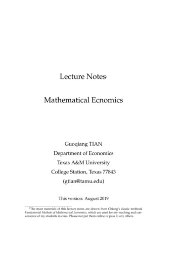
CHAPTER 3. EQUILIBRIUM ANALYSIS IN ECONOMICS16running examples throughout the course.3.2 Partial Market Equilibrium - A Linear ModelIn a static-equilibrium model, the standard problem is that of finding theset of values of the endogenous variables which will satisfy the equilibrium conditions of the model.Partial-Equilibrium Market ModelPartial-equilibrium market model is a model of price determination in anisolated market for a commodity.Three variables:Qd the quantity demanded of the commodity;Qs the quantity supplied of the commodity;P the price of the commodity.The Equilibrium Condition: Qd Qs .The model isQd QsQd a bp (a, b 0)Qs c dp (c, d 0)The slope of Qd b, the vertical intercept a.The slope of Qd d, the vertical intercept c.Note that, contrary to the usual practice, quantity rather than price hasbeen plotted vertically in the figure.One way of finding the equilibrium is by successive elimination of variables and equations through substitution.

3.2. PARTIAL MARKET EQUILIBRIUM - A LINEAR MODEL17Qd , Q saQd a - b P(demand)Q Qd QsQs - c d P(supply)(P, Q )OP1PP-cFigure 3.1:From Qs Qd , we havea bp c dpand thus(b d)p a c.Since b d ̸ 0, the equilibrium price isp̄ a c.b dThe equilibrium quantity can be obtained by substituting p̄ into eitherQs or Qd :Q̄ ad bc.b dSince the denominator (b d) is positive, the positivity of Q̄ requiresthat the numerator (ad bc) 0. Thus, to be economically meaningful,the model should contain the additional restriction that ad bc.

CHAPTER 3. EQUILIBRIUM ANALYSIS IN ECONOMICS183.3 Partial Market Equilibrium - A Nonlinear ModelThe partial market model can be nonlinear. Suppose a model is given byQd Qs ;Qd 4 p2 ;Qs 4p 1.As previously stated, this system of three equations can be reduced toa single equation by substitution.4 p2 4p 1,orp2 4p 5 0,which is a quadratic equation. In general, given a quadratic equation inthe formax2 bx c 0 (a ̸ 0),i

mathematical statistics. Therefore, it is of great necessity to master suffi-cient mathematical knowledge if you want to learn economics well, con-duct economic research and become a good economist. 1.2 Advantages of Mathematical Approach Mathematical approach has the following advantages: