Transcription
Excel IntermediateTable of ContentsFormulasUPPER, LOWER, PROPER AND TRM .2LEFT, MID, and RIGHT.3CONCATENATE .4& (Ampersand) .5CONCATENATE vs. & (Ampersand) .5ROUNDUP, and ROUNDDOWN .6VLOOKUP .7HLOOKUP.9IF .10Nested IF .11IF and AND .12SUMIF .13Error Values in Excel .14ChartsRibbon Tour .14Creating a chart .15Chart Layout Options.16Multiple Series within a chart .17Modifying Gridlines .21FiltersRibbon Tour .23Quick Filtering .23Filtering by multiple criteria .25Saving Filtered Data.27Text to Columns (Data Parsing)UPPER, LOWER, PROPER AND TRIM .28
FormulasUPPER, LOWER, PROPER, and TRIMThese formulas all work with text. After using one of these functions it is good practice to paste special\values sothat they will remain in their desired formatting.123UPPER, LOWER, PROPER, and TRIMFormulaDescription UPPERConverts all text to upper case LOWERConverts all text to lower case PROPERCapitalizes the first letter in a text string and any other letters intext that follow any character other than a letter, i.e. a space.Converts all other letters to lowercase TRIMRemoves all blank, unnecessary spaces at the start and end of astring including extra spaces, tabs, and other characters thatdon’t print.LEFT, MID, and RIGHTWhen data is imported or copied into an Excel spreadsheet unwanted characters or words can sometimes beincluded with the new data. Excel has several functions that can be used to remove such unwanted characters.Which function you use depends upon where the unwanted characters are located: If the unwanted characters are on the right side of your good data, use the LEFT function to remove them. If you have unwanted characters on both sides of your good data, use the MID function to remove them. If these unwanted characters appear on the left side of your good data, use the RIGHT function to removethem.2
LEFT, MID, and RIGHTFormulaSyntaxEnglish Translation LEFT LEFT(text, num chars)Using the piece of data you want, typically a cellreference, indicate how many characters you wantused/ brought back starting at the left mostposition. MID MID(text, start num,num chars)Using the piece of data you want, typically a cellreference, indicate the first character to be usedstarting at the left most position and how manycharacters to the right of the start number to beused/brought back. RIGHT RIGHT(text, num chars)Using the piece of data you want, typically a cellreference, indicate how many characters you wantused/ brought back starting at the rightmostposition.To increase the power of LEFT formula combine it with a FIND. Instead of counting the number of spaces you haveto move through the cell, key of a constant. Below is a screen shot of a listing of name, location, and gender. Thelocation includes both the city and state. The desire is to separate the city and state into two fields.In order to separate the city utilizing the LEFT command, there are a couple of options.1.2.The common one of specifiying the number of characters that it needs to move over. This is difficult dueto them being of different lengths.Or instruct the formula to bring back the characters after the FIND command locates what it is looking for.3
Utilizing the common LEFT will not work in this scenario because the length of the city names is not consistent.Redding in D1 is just fine; however Palo Cedro is cut off because it is longer.1By combining the FIND with the LEFT, you can quickly get exactly what you want. The negative one (1) is addedbecause if not, the comma would be returned as well.2CONCATENATEThe CONCATENATE function is used to join two or more words or text strings together. After using this function itis good practice to paste special\values so that they will remain in their desired formatting.The syntax is CONCATENATE(A1,B1,C1 .)The finished product is quite literally a combination of the text without any spaces. If spaces are desired, there aretwo options. The first to add within your formula the cell reference where there is a space as the only value withinthe cell value, or to add a space within the formula. Since text is being added, it must be lead and followed by adouble quote (“). An example is CONCATENATE(A1,” “,B1,” “,C1).An example of CONCATENATE is below and combined with & due to their interchangeability.4
& (Ampersand)The & connects, or concatenates, multiple values to produce one continuous text value. After using this function itis good practice to paste special\values so that they will remain in their desired formatting.CONCATENATE vs. & (Ampersand)Besides CONCATENATE sounding smarter, and worth fifteen points in Scrabble, the two functions areinterchangeable and really come down to personal preference. CONCATENATE formulas tend to be a bit easier toread.Either function may be used to combine words or phrases that are not part of the range. For instance, we want tofill in the blanks for the following sentence:Famous February birthdays are and .And we have the following data table:5
By utilizing the CONCATENATE formula, we can substitute text located in cells within our spreadsheet into acompleted sentence.ROUNDUP and ROUNDDOWNThe ROUNDUP function is used to round a number upwards toward the next highest number. Although similar toROUND, ROUNDUP always rounds upward whereas ROUND will round up or down depending on whether the lastdigit is greater than or less than five (5).Although the ROUNDUP can be a standalone formula, it is often nested with other formulas, for example SUM. It isespecially useful with division due to the fractions that are often created.6
VLOOKUPThe VLOOKUP function searches vertically (top to bottom) the leftmost column of a table until a value thatmatches or exceeds the one you are looking up is found.The elements being looked up must be unique and must be arranged or sorted in ascending order; that is,alphabetical order for text entries, and lowest‐to‐highest order for numeric entries.The syntax is VLOOKUP(lookup value,table array,col index num,[range lookup]).An example of the formula is: VLOOKUP(E2,D2:M3,2,TRUE) The English translation is using the value found in thecell E2, look in the range of D2 to M3 row by row. If you find a value that matches or exceeds the value in E2,using that row, go over 2 columns to the right, grab the value there and bring it back.There are two range lookup argument options; TRUE or FALSETRUEIs the default answer, so you may leave it out of the formulaLooks for an approximate matchIf it finds an exact match it will use it.If it doesn’t find an exact match, it will use the last item before it got greaterAlphabetical: Looking for Cat. If elements are Apple, Bird, Carpet, Dog; then Carpetwould be returned because Dog exceeds Cat alphabetically.Numeric: Looking for 5.25. If elements are 3.0, 4.0, 5.0, 6.0, 7.0, then 5.0 would be used.The last number before 5.25 was exceeded.FALSELooks for an exact match.If it finds an exact match it will use it.If it doesn’t find an exact match, it will return #N/AAlphabetical: Looking for Cat. If elements are Apple, Bird, Carpet, Dog; then #N/A wouldbe returned.Numeric: Looking for 5.25. If elements are 3.0, 4.0, 5.0, 6.0, 7.0, then #N/A would bereturned because there is no exact match.7
8
HLOOKUPThe HLOOKUP function searches horizontally (left to right) the topmost column of a table until a value thatmatches or exceeds the one you are looking up is found.The elements being looked up must be unique and must be arranged or sorted in ascending order; that is,alphabetical order for text entries, and lowest‐to‐highest order for numeric entries.The syntax is HLOOKUP(lookup value,table array,row index num,[range lookup])An example of the formula is: HLOOKUP(E2,D2:M3,2,TRUE) The English translation is using the value found in thecell E2, look in the range of D2 to M3 and go column by column. If you find a value that matches or exceeds thevalue in E2, using that row, go down 2 rows to the right, grab the value there and bring it back.There are two range lookup argument options; TRUE or FALSETRUEIs the default answer, so you may leave it out of the formulaLooks for an approximate matchIf it finds an exact match it will use it.If it doesn’t find an exact match, it will use the last item before it got greaterAlphabetical: Looking for Cat. If elements are Apple, Bird, Carpet, Dog; then Carpetwould be returned because Dog exceeds Cat alphabetically.Numeric: Looking for 5.25. If elements are 3.0, 4.0, 5.0, 6.0, 7.0, then 5.0 would be used.The last number before 5.25 was exceeded.FALSELooks for an exact match.If it finds an exact match it will use it.If it doesn’t find an exact match, it will return #N/AAlphabetical: Looking for Cat. If elements are Apple, Bird, Carpet, Dog; then #N/A wouldbe returned.Numeric: Looking for 5.25. If elements are 3.0, 4.0, 5.0, 6.0, 7.0, then #N/A would bereturned because there is no exact match.9
IFThe formula makes a statement/question, if the answer is true then one response is obtained. If the answer iffalse, then another answer is obtained.The syntax is IF(logical test,value if true,value if false)The formula is IF(G6 0, ”Have money left to spend.”,”Houston, we have a problem”). The English translation is ifthe value found in G6 is greater than zero THEN display the comment ‘Have money left to spend.ELSE display thecomment ‘Houston, we have a problem’.Nested IFA nested IF command is merely multiple if statements within the same formula.The formula is IF(G8 0, ”Have money left to spend.”,IF(G8 ‐5000,”We are in it deep!”,”Houston, we have aproblem”). The English translation is if the value found in G8 is greater than zero THEN display the comment ‘Havemoney left to spend.’ IF it is less than Negative 5,000 then display ‘We are in deep!’ ELSE display the comment‘Houston, we have a problem’.IF & ANDThe AND function is a logical function which generates an output of either TRUE or FALSE. By itself, the ANDfunction has limited usefulness. However, combining it with other functions, such as the IF, greatly increases thecapabilities of a spreadsheet.10
The syntax is of the IF is: IF(logical test,value if true,value if false) and the syntax of the AND is: AND(logical1,logical2, ) with only one logical being required. With that being said the combined syntax is simply the ANDreplacing the logical test parameter: if(AND(logical1, logical2, ,value if true,value if false).The formula is IF(AND(D10 C10,G10 0),”We made a bad budget adjustment”,”Budget adjustment was a goodone’). The English translation is IF the revised budget is less than the Adopted budget AND account balance is lessthan zero THEN display ‘We made a bad budget adjustment’ ELSE display ‘Budget adjustment was a good one.’SUMIFWhat about those times when you only want the total of certain items within a cell range? For those situations,you can use the SUMIF function. The SUMIF function enables you to tell Excel to add together the numbers in aparticular range only when those numbers meet the criteria that you specify. The syntax of the SUMIF function isas follows: SUMIF(range
Excel has several functions that can be used to remove such unwanted characters. Which function you use depends upon where the unwanted characters are located: If the unwanted characters are on the right side of your good data, use the LEFT function to remove them.