Transcription
Excel Proficiency ExercisesWith suggested solutionsEXCEL REVIEW2001-2002
The best way to learn Excel is to use it.The best way to use Excel is on the jobto solve a problem you need solvingor by devising your own problems andfinding solutions to them. This documentincludes practice exercises thatillustrate features of the Excel software thatare useful for modeling problems.Thanks to Decision Science Professor Laura Kornishfor suggesting the exercises in this document.Try solving each problem on your own.If you need help, notes and suggested solutionsare included. You may come up with solutionsthat use different techniques and that look a bit differentfrom the ones here; your solutions may be completelyvalid! Excel offers many ways to accomplish the same thing.Paula EcklundSpring 2001
ContentsPage1. Multiplication Table Problem.1Relative, Absolute, & Mixed Addressing2. Olive Oil Pricing Problem.6IF Statements, SUMPRODUCT Function, MIN Function3. Web Service Problem.13Forecasting & Charting4. Pro Forma Problem.19Forecasting, Data Table, Goal Seek5. Data Relationship Problem .28Scatter or XY Plot
THIS PAGE INTENTIONALLY BLANK.
1. Multiplication Table ProblemRelative, Absolute, and Mixed AddressingThe ExerciseCreate a 10x10 multiplication table in a spreadsheet, as shown below. The cells inside thetable (i.e., within the black border) should contain only formulas, not numbers. Youshould find it unnecessary to enter more than a single formula, which can be dragcopied to fill the rest of the 24048566472809 109 1018 2027 3036 4045 5054 6063 7072 8081 9090 100NotesThe principle behind completing this multiplication table is simple. You want a formulain each cell of the table matrix that multiplies the value in that cell’s column header bythat cell’s row header. The trick is to write a single formula (a “master formula”) that canbe copied into all the matrix cells and is valid for each one.Solving this problem by writing a single formula requires that you understand Excel’smixed addressing feature. Note that mixed addressing comes into play only when aformula is copied, as we’re doing here. So that’s the only time you need to concernyourself with it.Before you tackle mixed addressing, you should first understand Excel’s relatedaddressing options: relative and absolute. Excel’s default is relative addressing. That is,cell references contained within a formula that’s copied are adjusted in the copy relativeto their position in the spreadsheet. Fixed addressing is the opposite. As its nameimplies, a fixed reference, when copied as part of a formula, does not change.Excel uses a dollar sign ( ) to indicate that a reference is fixed. For example, the cellreference A1 (without dollar signs) is relative, whereas A 1 (with dollar signs) is fixed.Mixed addressing occurs when either the column reference or the row reference is fixed,but not both. For example, A1 is a mixed reference where the column A is fixed but notthe row and A 1 is a mixed reference where the row 1 is fixed but not the column.For our multiplication table problem, it will satisfy the requirements of the upper-lefthand cell of the matrix if we write a formula that multiplies the value in the column1
header by the value in the row header. So, for example, our initial formula might looklike this: B1*A2and the result in the matrix would Using Relative AddressingIf we copy that formula to the rest of the matrix, however, the results are not what weintended, as shown in the partial view 205040403203628803628800242457669120497664002.51E 111.01E 163.67E 211.33E 286245763317762.29E 101.14E 182.86E 292.89E 451.06E 671.41E 95245763317761.1E 112.52E 212.88E 398.25E 682.4E 1142.5E 1813.6E 276120691202.29E 102.52E 216.37E 421.84E 821.5E 1513.6E 265#NUM!#NUM!Where we’ve gone astray is in copying the original formula with no thought to theimpact of relative addressing on the copies of the original formula. By default, Excel hasused relative addressing in all the copies, adjusting cell references in the formula foreach new formula location. So reading down the first column, the formulas are: B1*A2 B2*A3 B3*A4 B4*A5and so on2
and in the second column, the formulas are: C1*B2 C2*B3 C3*B4 C4*B5and so on.Even though the original formula gave the correct value for the upper-left-hand cell ofthe matrix, that formula was insufficient when we wanted to copy it to fill the rest of thematrix cells.So how can we properly fill the matrix? One way is to write an individual formula foreach cell in the matrix. But the much more efficient way called for in this exercise is tomodify the relative cell references in the original formula before copying it so eachcopied formula references the correct values for its location in the matrix.Using Absolute AddressingIf the original formula is B1*A2 then which references shall we fix? Making both cellreferences absolute, the formula becomes B 1* A 2. However, the result of copyingthat formula is incorrect, putting exactly the same formula in each cell of the matrix:A1234BC1111123D2111E3111F41115111So using absolute addressing in this case doesn’t work either.Using Mixed AddressingInstead of using relative or absolute addressing, mixed addressing will solve ourproblem. Imagine that we start by copying the original formula from the upper-lefthand cell down the first (left-hand) column. In the first cell reference of the originalformula (B1) we need to fix the row 1, but not necessarily the column B. So that adjustedcell reference reads B 1 and the formula reads B 1*A2. Copying that formula down thefirst column yields correct answers in the first column. So far so good.A1234567B123456C1123456D23E3F45
The next step is to copy the formulas in the first column to the columns to their right.When we do so the values in the second column (column C) look OK, but thesubsequent columns contain incorrect values.A1234567B123456C1123456224681012DEF3456 24 12012 48 24018 72 36024 96 48030 120 60036 144 720Again, our downfall is relative addressing, this time in the second cell reference of theformula. Looking in column F, for example, the copied formulas read: F 1*E2 F 1*E3 F 1*E4and so on.Using Mixed Addressing CorrectlyTo correct this error, we go back to the original formula. In that formula, the second cellreference must be fixed as to column. So the formula B 1*A2 must be adjusted to read B 1* A2. Copying this corrected formula from the upper-left-hand cell to the rest ofthe cells in the matrix results in correct values in all the 4324048566472809 109 1018 2027 3036 4045 5054 6063 7072 8081 9090 100For more information on relative, fixed, and mixed addressing see Excel’s online help on the topicMove or copy a formula.4
The “Multiplication” tab from the Solutions.xls workbook.5
2. Olive Oil Pricing ProblemIF Statements, SUMPRODUCT Function, MIN FunctionThe ExerciseOlive oil can be purchased according to this price schedule:For the first 500 gallonsFor any of the next 500 gallonsFor any oil beyond 1,000 gallons 23 per gallon 20 per gallon 15 per gallonCreate a spreadsheet that will calculate the total price of buying x gallons of oil, where xis a number to be entered into a cell on the spreadsheet.NotesCreating this spreadsheet requires the use of Excel’s powerful IF statement. The syntaxof the IF statement is a three-part “if-then-else” format. If the test condition (the firstparameter) evaluates to true, the value-if-condition-true (the second parameter) isreturned. But if the test condition evaluates to false, the value-if-condition-false (thethird parameter) is returned. IF(condition-to-test, value-if-condition-true, value-if-condition-false)A simple example: IF(Sky-is-blue, sunny-day, cloudy-day)IF statements can be nested, although to retain clarity in your work it’s generally not agood idea to nest them to very many levels. A nested IF statement (where the nested IFtakes the place of the value-if-condition-false in the original IF statement) might look likethis: IF(condition-to-test, value-if-condition-true, IF(condition-to-test, value-ifcondition-true, value-if-condition-false))Continuing our weather example, a nested IF statement might read like this: IF(Sky-is-blue, sunny-day, IF(Temp 32, Maybe-snow, Maybe-rain))The olive oil pricing exercise specifies three oil prices based on quantity ( 23/gallon forup to 500 gallons, 20/gallon for 501-1,000 gallons, and 15/gallon for 1,001 or moregallons) and has as its variable x gallons of oil to buy.An Initial, Simple ScenarioThe Solutions.xls spreadsheet begins by presenting a solution to a simpler version of theexercise that requires only a single IF statement. This version supposes 3 values for xthat account for three quantity possibilities (1,600, 483, and 2001 gallons). But instead ofthree pricing levels, the simpler version has only two: first 500 gallons and any amountover 500. Because there are only two pricing levels in this version, a simple IF statementcan be used to calculate the cost at these three levels.6
If the price schedule were:first500 gallons at additionalgallons at Cost ofCost ofCost of1600 gallons is483 gallons is2001 gallons is23.0020.00 33,500.00 11,109.00 41,520.00Assigning names to key variables makes it easier to read the IF formula. I’ll assign thesenames:Quantity1to the cell for gallons that holds 1,600Price for 500to the cell for price that holds 23.00First500to the cell for quantity that holds 500Price for Over500 to the cell for price that holds 20.00If the price schedule were:first500 gallons at additionalgallons at Cost ofCost ofCost of1600 gallons is483 gallons is2001 gallons is23.0020.00 33,500.00 11,109.00 41,520.00Then we can write an IF statement that reads like this: IF(Quantity1 First500,Price for 500*Quantity1, First500*Price for 500 (Quantity1-First500)*Price for Over500)Below is the same formula but formatted and with then and else added to better see theIF logic: IF(Quantity1 First500,then Price for 500*Quantity1,else First500*Price for 500 (Quantity1First500)*Price for Over500)The result of the IF statement for 1,600 gallons is 33,500.00. If you insert absolute (ormixed) addressing in the first formula where needed, you can copy the first IF statementdown the column to also solve for the given quantities of 483 and 2,001 gallons.The Actual Problem ScenarioThe second scenario on the “Oil prices” tab of the Solutions.xls spreadsheet is morecomplex and reflects the actual problem. In this scenario, there are three price levels (nottwo) with any amount over 1,000 gallons priced at 15.00/gallon. Again, the challenge is7
to construct a single formula that can handle the three-tier pricing structure for anyquantity.For the price schedule in the problem:first500 gallons at 23.00next500 gallons at 20.00any additionalgallons at 15.00Cost ofCost ofCost of1600 gallons is483 gallons is2001 gallons is 30,500.00 11,109.00 36,515.00For this more complex variation, we use a nested IF statement along with Excel’s built-inSUMPRODUCT function. For example, the formula to calculate the cost of 1,600 gallonsmakes use of the cell values marked by rectangles in the illustration below:Again, naming cells to make our formula easier to follow:Quantity1 is the name of the cell for gallons that holds 1,600Price for 500 names the cell for price that holds 23.00Price for 500 names the cell for price that holds 20.00Price for 1K names the cell for price that holds 15.00First500 names the cell for quantity that holds 500Next500 names the cell for quantity that holds the 2nd 500Then to solve for cost we write a nested IF formula that reads like this: IF(Quantity1 First500,Price for 500 * Quantity1,IF(Quantity1 SUM(First500, Next500),First500*Price for 500 (Quantity1-First500)*Price for 500,SUMPRODUCT (First500:Next500,Price for 500:Price for 500) (Quantity1 SUM(First500,Next500)*Price for 1K))We can then copy this formula to solve for the two other quantities given: 483 gallonsand 2,001 gallons.8
A Closer Look at the SUMPRODUCT Part of the FormulaAlong with using a nested IF statement, our formula also makes use of the powerfulExcel built-in function named SUMPRODUCT. The syntax for the SUMPRODUCTfunction is: SUMPRODUCT(array1,array2,array3, )The SUMPRODUCT part of our formula reads like this:SUMPRODUCT(First500:Next500, Price for 500:Price for 500)and means: Multiply First500 by Price for 500 (or 500* 23.00) to get value1. Multiply Next500 by Price for 500 (or 500* 20.00) to get value2. Add together value1 and value2.As you can see, the SUMPRODUCT function takes two or more arrays as its parameters.It multiples the first value in the first array by the first value in the second array, thesecond value in the first array by the second value in the second array, and so on. Whenall the multiplication operations across arrays are complete, the results are addedtogether.An Alternative Calculation MethodAs is generally always the case with Excel, there’s more than one good way to modelthis problem. The Solutions.xls worksheet shows an alternative method that againmakes use of nested IF statements and SUMPRODUCT as well as the MIN function.9
1
Excel Proficiency Exercises With suggested solutions EXCEL REVIEW 2001-2002. The best way to learn Excel is to use it. The best way to use Excel is on the job to solve a problem you need solving or by devising your own problems and finding solutions to them. This document includes practice exercises that illustrate features of the Excel software that are useful for modeling problems. Thanks to .File Size: 469KBPage Count: 38
