Transcription
MIMO I: Spatial DiversityCOS 463: Wireless NetworksLecture 16Kyle Jamieson[Parts adapted from D. Halperin et al., T. Rappaport]
What is MIMO, and why? Multiple-Input, Multiple-Output (MIMO) communications– Sends and receive more than one signal on different transmitand receive antennas We’ve already seen frequency, time, spatial multiplexing in 463:– MIMO is a more powerful way to multiplex wireless mediumin space– Transforms multipath propagation from an impediment toan advantage2
Many Uses of MIMO At least three different ways to leverage space:1. Spatial diversity: Send or receive redundant streams ofinformation in parallel along multiple spatial paths– Increases reliability and range (unlikely that all paths will bedegraded simultaneously)2. Spatial multiplexing: Send independent streams ofinformation in parallel along multiple spatial paths– Increases rate, if we can avoid interference3. Interference alignment: “Align” two streams of interferenceat a remote receiver, resulting in the impact of just oneinterference stream
MIMO-OFDM(5) QPSK ModulatedSymbolssubcarriersf(6) Mapped onto Subcarriers as OFDM Symbolaphicalview offading:the OFDMthe 18 Mbps rate (QPSK, 3/4) Multipathdifferentencodingeffects onprocessdifferentforfrequencies) are encoded by a rate-1/2 convolutional code (1) and then optionally punctured b– OFDM: Orthogonal Frequency Domain Multiplexinghigher coding rates (here, 3/4) that send fewer redundant bits (2). The remainingDifferentsubcarriersindependentof each otherspread–theredundancyacrossaresubcarriersand protectagainst frequency-selective fainto symbols (4) based on the modulation (QPSK encodes 2 bits per symbol), modpedthe di erent ontoChannelmodel forsubcarriersOFDM: y toh xform w an OFDM symbol (6).h11– A single complex number h captures the effect of the channel on datah11h11h11 xy1 h11x 1y ( h11 h21) xiny1 a particularsubcarrierxx1h12h21 h For MIMO:Think about each subcarrier, independentof other subcarriersRxRxTx12h21TxxRxx2h22
Plan1. Today: Diversity in Space– Receive Diversity– Transmit Diversity2. Next time: Multiplexing in Space3. Next time: Interference Alignment5
Path Diversity: Motivation1. Multi-Antenna Access Points (APs), especially 802.11n,ac:2. Multiple APs cooperating with each other:Wired backhaul3. Distributed Antenna systems, separating antenna from AP:Antenna 1APAntenna 2Coaxial / Fiberbackhaul6
Review: Fast Fading Typical outdoor multipath propagation environment, channel h On one link each subcarrier’s power level experiences Rayleigh fading:!"7
Uncorrelated Rayleigh Fading Suppose two antennas, separated by distance d12 Channels from each to a distant third antenna (h13, h23) can be uncorrelated– Fading happens at different times with no bias for a simultaneous fade!" # , !##8
When is Fading Uncorrelated, and Why? ,!"# Channels from each antenna (h13, h23) to a third antenna– Channels are uncorrelated when !"# &. ()– Channels correlated, fade together when !"# ) This correlation distance depends on the radio environmentaround the pair of antennas– Increases, e.g., atop cellular phone tower9
Plan1. Today: Diversity in Space– Receive Diversity Selection Diversity Maximal Ratio Combining– Transmit Diversity2. Next time: Multiplexing in Space3. Next time: Interference Alignment10
Channel Model for Receive Diversity One transmit antenna sends a symbol to two receive antennas– Receive diversity, or Single-Input, Multi-Output (SIMO)h1xxh2p9/ 13y1 3ei3π/4xReceive antenna 1protate, scale by 3/ 13pn1p4/ 13Receive antenna 2n2protate, scale by 2/ 131n expected 1y2 2e-iπ/6xFigure 3: MRC operation on a sample channel. The channel gains are h h3ei3 /4 , 2e i /6 i, witre 1: Agraphical view of the OFDM encoding process for the 18 Mbps rate (Qnoise n hn1 , n2 i of expected power 1. The antennas have respective SNRs of 9 and 4. To implemdata bitsare encodedbyreceiveda rate-1/2(1) andthenoptionally h / h , h denotes tpthe(0)receivermultiplies thesignalconvolutional y hx n by the codeunit vectorwhereain bits conjugatefor highercodingrates (here,3/4)antenna’sthat sendfewerbitsrotates(2). Theof h.This operationscales eachsignalby itsredundantmagnitude, andthephasethereferencebefore addingthem.(For graphicalclarity,we depictthe commonphasaved otectagainstfrequencyprather intothan symbolsat 0). The resultingsumonhasthemagnitude13, andexpectedencodesnoise power1 becausethare grouped(4) basedmodulation(QPSK2 bitsper synormalized. Thus, by coherently combining received signals from di erent antennas, the MRCfinally mappedontothedi erentsubcarriersforman OFDMsymbol(6).subcarrthe expectedSNRof 13.In systemswith OFDM, toMRCis performedseparatelyfor each Each receive antenna gets own copy of transmitted signal via– Different path– Potentially different channel
Selection Diversityh1xxh2p9/ 13y1 3ei3π/4xRx 1protate, scale by 3/ 13Select strongern1Rx 2n2p4/ 13Radioprotate, scale by 2/ 13p13n expected 1y2 2e-iπ/6x i3 /4i /6Figure 3: MRC operation on a sample channel. The channel gains are h h3e, 2ei, with GaussiaAgraphicalviewof thepowerOFDMencodingprocessforSNRsthe of189 Mbpsrate(QPSK,3noise n mplementMRC12 Tworeceivebyantennasshare one receivingradioshe(0)are encodeda rate-1/2(1)andthenoptionallypunctur h / h , h denotes thereceivermultiplies thereceivedsignalconvolutional y hx n by the codeunit vectorwherecomple ntbits(2).Theremainconjugate of h. This operation scales each antenna’s signal by its magnitude, and rotates the signals inthephasethereferencebefore addingthem.(For graphicalclarity,we depictthe commonphase verticallyto ersignal,sendsthattotheradioratherthan symbolsat 0). The resultingsumonhasthemagnitude13, andexpectedencodesnoise power1 becausethe scaling iped into(4) basedmodulation(QPSK2 bitsper symbol),normalized.Thus, byreliabilitycoherently combiningreceived bad)signals from di erent antennas, the MRC output ha– ontoHelps(bothunlikelymappedthedi erentsubcarriersforman OFDMsymbol(6).subcarrier.he expectedSNRof 13.In systemswith OFDM, toMRCis performedseparatelyfor eachhh11 This is yknownx a 1x2 system. Real systems11econd node.1 h11 asmay have more than two receive antennas, but xtwo will suffice for our explanation. With this setup, each receive anenna receives a copy of the transmitted signal modified byer (dB)– Wastes received signal from other antenna(s)y 0( h11 h21) x-5x1h11h12y1 h21
Selection Diversity:Performance Improvement In general, might have M receiveantennas (average SNR Γ)– !" : SNR of the i th receive antenna Probability selected SNR is lessthan some threshold γ:– Pr !%, , !( γ Pr !" γProbability (%) that SelectedAntenna’s SNR Exceeds Threshold γ( One more “9” of reliability peradditional selection branchHigher probability(better) ß lower threshold SNR13
Leveraging All Receive Antennash1xxh2p9/ 13y1 3ei3π/4xRx 1protate, scale by 3/ 13pn1n2Rx 2protate, scale by 2/ 13p4/ 1313n expected 1y2 2e-iπ/6xFigure3: MRCtooperationon thea sampleThesignalschannel gainsh h3e, 2ei, with Gaussia Wantjustofaddtwo sstogetherforarethe18 Mbpsrate(QPSK, 3noise n hn1 , n2 i of expected power 1. The antennas have respective SNRs of 9 and 4. To implement MRCshe(0)areencodedbya therate-1/2code(1) andthenoptionallypunctur h / out h , h denotes the– Butif eceivedsignalconvolutional y hx n by theunit vectorwherecomple ntbits(2).Theremainconjugate of h. This operation scales each antenna’s signal by its magnitude, and rotates the signals inthephasethereferencebefore addingthem.(For graphicalclarity,we depictthe commonphase ndprotectagainstfrequency-selectivpratherthanat 0). Theresultingsumhasthemagnitudeandexpectednoise thenpower1addbecausethe scaling i intoSolution:ReceiveM onradios,align13,signalphases,pedsymbols(4) basedmodulation(QPSKencodes2 bitsper symbol),normalized. Thus, by coherently combining received signals from di erent antennas, the MRC output hamappedthedi erentsubcarriersan OFDMsymbol(6).subcarrier.– ontoRequiresMsystemsreceiveinformgeneralhe expectedSNRof 13.Inwithradios,OFDM, toMRCis performedseparatelyfor eachhh11 This is yknownx a 1x2 system. Real systems11econd node.1 h11 asmay have more than two receive antennas, but xtwo will suffice for our explanation. With this setup, each receive anenna receives a copy of the transmitted signal modified byer (dB) y 0( h11 h21) x-5i3 /4x1i /6h11h12y1 h21
How to Choose Weights?h1xxh2p9/ 13y1 3ei3π/4xRx 1protate, scale by 3/ 13n1n2Rx 2protate, scale by 2/ 13yp4/ 13p13n expected 1y2 2e-iπ/6xFigure3: MRC operationona sample channel.Thechannelgains areish! h3e, 2ei, with Gaussia Supposephaseof incomingon thei branchAgraphicalviewof theOFDM signalencodingprocessfor the "18 Mbpsrate(QPSK, 3noise n hn1 , n2 i of expected power 1. The antennas have respective SNRs of 9 and 4. To implement MRCshe(0)are encodedbyreceiveda rate-1/2(1) andthenoptionallypunctur h / h , h denotes thereceivermultiplies thesignalconvolutional y hx n by the codeunit vectorwherecomple( , ntbits(2).Theremain.conjugateh. Thisscalesleteachsignalby its# magnitude,the signals int To ofalign{ yioperation} in phase,theantenna’scombineroutput "&' )"and* rotateshephasethereferencebefore addingthem.(For graphicalclarity,we depictthe commonphase mplitudesa?ratherthan symbolsat 0). The resultingsumonhasthemagnitude13, andexpectedencodesnoise power1 becausethe scaling iiped into(4) basedmodulation(QPSK2 bitsper symbol),normalized. Thus, by coherently combining received signals from di erent antennas, the MRC output hamappedontothedi erentsubcarriersforman OFDMsymbol(6).subcarrier.he expectedSNRof 13.In systemswith OFDM, toMRCis performedseparatelyfor eachth i3 /4i /6Idea: Put more weight into branches with high SNR: Let /0 10h–11 Thish11yknown h11 asx aMaximal0( h11 h21) xCombiningy (MRC)econd node.This isis1x2 system. RatioReal systems1 calledmay have more than two receive antennas, but xtwo will suf-fice for our explanation. With this setup, each receive anenna receives a copy of the transmitted signal modified byer (dB) x1-5h11h12y1 h21
MRC: Performance ImprovementProbability that MRC’s SNR is Under Threshold γ0010 110PoutM 1 210M 2M 3 310M 4Lower probability(better) M 10M 20 410 10 50510152010log'( )/ (10log (γ/γ )10025303540Lower threshold SNR àFigure 7.5: Pout for MRC with i.i.d. Rayleigh fading. Two “9”sof reliability improvement between one (i.e., no MRC) and twoRayleigh fading, where pγ (γ) is given by (7.16), it can be shown that [4, Chapter 6.3]MRC branchesΣPb !0 "Q( 2γ)pγΣ (γ)dγ #1 Γ2&'# M M 1%1 Γ mM 1 mm 0m2,(7.18)16
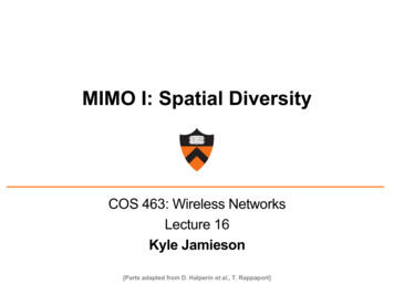
d power 1. The antennas have respective SNRs of 9 and 4. To implement MRC,eceived signal y hx n by the unit vector h / h , where h denotes the complextion scales each antenna’s signal by its magnitude, and rotates the signals intofore adding them. (For graphicalclarity, we depict the common phase vertically,plting sum has magnitude 13, and expected noise power 1 because the scaling isrently combining received signals from di erent antennas, the MRC output hassystems with OFDM, MRC is performed separately for each subcarrier.a 1x2 system. Real systemsantennas, but two will sufthis setup, each receive annsmitted signal modified bymitter and itself. The chaners that represent both thechannel as well as the pathe 3 for a graphical example).nel gains based on trainingote that the gains di er forective fading) as well as forw is how to combine the twoe of them.niques to show the extremes.e antenna with the strongesto receive the packet and igs method SEL, for selectionat is done by 802.11a/g APsps with reliability, becausebad, but it wastes perfectlynnas that are not chosen.d the signals from the twos cannot be done by simplywe will have just recreatedRather, the signals shouldn the same phase; then, thene coherently. To do this,F chain for each antenna toes the hardware complexity Normalized power (dB)Selection Diversity, in Frequency0-5-10-15ACB and SELAB (MRC)ABC (MRC)-20-25-20-1001020Subcarrier indexFigure 4: Frequency-selective fading over testbedAntennas A and links:C he figure shows,for an exampleGHzlink,the received power measured on each subcarrier forindividual antennas and under SEL and MRC diversity, normalized to the strongest subcarrier power.Selection Combining (“SEL”) improves but certain subcarriers still experience fadingtudes of 3 and 2. With expected noise power 1, these gainscorrespond to SNRs of 9 and 4, given that a signal’s power isthe square of its magnitude. The MRC receiver scales eachantenna’s signal by its magnitude, normalized to the total;delays the signals to a common phasepreference; and thenadds them. The result has magnitude 13, and the normalized weighted sum of noise still has expected power 1. TheMRC increases power and flattens nulls, leading to fewer bit errors
MRC’s Capacity Increase MRC with M branches increases SNR– Increased Shannon capacity Sub-linear (logarithmic) capacity increase in M:– !"# &' ( log 1 . ( /01 bits/second/Hz
Plan1. Today: Diversity in Space– Receive Diversity– Transmit Diversity Channel reciprocity Transmit beamforming Introduction to Space-Time Coding: Alamouti’s Scheme2. Next time: Multiplexing in Space3. Next time: Interference Alignment19
An Aside: Radio Channels are “Reciprocal”a2,d2,τ2Transmitter Ta1,d1,τ1Receiver R Forward channel (T to R) is ℎ"# %& '()* ,/. %)'()* 0/. Switch T and R roles, changing nothing else:– Reverse channel (R to T) is ℎ#" %& '()* ,/. %)'()* 0/. ℎ"#– The reverse radio channel is “reciprocal” Practical radio receiver circuitry induces differences between ℎ"# , ℎ#"20
Transmit Diversity: Motivation More space, power, processing capability available at thetransmitter?– Yes, likely! e.g. Cellular base station, Wi-Fi AP transmittingdownlink traffic to mobile But, a (possible) requirement: May need to know the radiochannel at the transmitter before the transmission commences– cf. receive diversity: channel from preamble reception Then, a tension: Separate transmit antennas for path diversity– Antenna 1, Antenna 2, transmit radio non co-located Then, harder to move transmit signals, radio channel measurementsi.e. channel state information (CSI) between the three locations21
Transmit Beamforming: Motivation“receiver” Suppose the transmitter knows the CSI to receivers Transmitters align their signals so that constructiveinterference occurs at the single receive antenna– Align before transmission, not after reception (receivebeamforming)22
Transmit Beamforming Leverage channel reciprocity, receive beamforming “in reverse” Send one data symbol x from two antennas,'()y1% 3e# &i3π/4xxp9/ 13ℎ# %# & '(p)rotate,scaleby3/13Tx 1n1n2'( Tx scale2 by 2/pℎ13*rotate,p &4/ %13#pReceive13 n expected 1-iπ/6y2 2e,'(x%* & MRC operation on a sample channel. The channel gains are h h3ei3 /4 , 2e i /6 i, with Gaussian1 , n2 i of expected power 1. The antennas have respective SNRs of 9 and 4. To implement MRC,multiplies the received signal y hx n by the unit vector h / h , where h denotes the complexf h. This operation scales each antenna’s signal by its magnitude, and rotates the signals intoase reference before adding them. (For graphicalclarity, we depict the common phase vertically,pat 0). The resulting sum has magnitude 13, and expected noise power 1 because the scaling is Multiply (pre-code) x by the complex conjugate of each channel23
Plan1. Today: Diversity in Space– Receive Diversity– Transmit Diversity Channel reciprocity Transmit beamforming Introduction to Space-Time Coding: Alamouti’s Scheme2. Next time: Multiplexing in Space3. Next time: Interference Alignment24
Alamouti Scheme: Motivation Suppose transmitters don’t know CSI information to receiver:what to do?1. Naïve beamforming (just send same signals)– Signals would often cancel out2. Repetition– Each antenna takes turns transmitting same symbol Receiver combines coherently– Use M symbol times Increases diversity (“SNR” term in Shannon capacity) Cuts Shannon rate by 1/M factor25
Alamouti Scheme Scope: A two-antenna transmit diversity system (M 2) Sends two symbols, s1 and s2, in two symbol time periods:Symbol Time PeriodAntenna 1:Antenna 2:1Send !"Send ! 2Send ! Send !" Then, by superposition the receiver hears:Symbol Time PeriodReceiver hears:1ℎ"!" ℎ ! 2 ℎ"! ℎ !" 26
Alamouti Receiver ProcessingSymbol Time PeriodReceiver hears:1y[1] ℎ'(' ℎ*(* [1]ℎ' [2]ℎ*2 [2] ℎ'(* ℎ*(' 2 ℎ* (' ℎ' (*ℎ* (' ℎ' (* Rewrite into two equations in two unknowns (s1 and s2):– (Receiver has CSI information)('ℎ' (* ℎ* ℎ* [1] ℎ' [2] But, what’s happening in terms of the physical wireless channel?27
Intuition for Alamouti Receiver Processing Start with the inverted channel matrix:!"& "# ℎ &( ,[1] ℎ , [2] Consider the computation for s1:– Rotate ,[1] by 1"– Rotate , [2] by 1(– Sum the result28
Alamouti: Impact of Phase Rotations Consider the computation for s1:– Rotate ![1] by &'– Rotate ! [2] by &*– Sum the resultSymbol Time PeriodReceiver hears:Phase after rotation:1y[1] ℎ./. ℎ1/1 2&* &'2! 2 ℎ1 /. ℎ. /1 2&* &'29
Alamouti: Receiver-Side PictureSymbol Time PeriodReceiver hears:Phase after rotation: 1y[1] ℎ'(' ℎ*(* /01 022 2 ℎ* (' ℎ' (* /01 02Receiver then sums all terms above:Received signal:Q 4* 4's2s2s1 s1I30
Alamouti: Interpretation!"ℎ" !# ℎ# ℎ# ([1] ℎ" ( [2]H Two new signal dimensions:1. Multiply two received symbols by the top column of H– Name this dimension ℎ" ℎ# – s1 arrives along this dimension (only!)2. Multiply two received symbols by the lower column of H– Name this dimension ℎ# ℎ" – s2 arrives along this dimension (only!)31
Alamouti: Performance Two dimensions: ℎ" ℎ % , ℎ ℎ"%Receivedsignal:Qs1 s1I Send half power on each antenna– For both symbols, '() , .-/ , . 0. Rate gain from enhanced SNR, and maintains one symbol persymbol time32
Multi-Antenna Diversity: Summary Leverage path diversity– Decrease probability of “falling into” to deep Rayleigh fade ona single link Defined new “dimensions” of independent communicationchannels based on space33
Thursday Topic:MIMO II: Spatial MultiplexingFriday Precept:Exploiting Doppler34
the received power measured on each subcarrier for individual antennas and under SEL and MRC diver-sity, normalized to the strongest subcarrier power. tudes of 3 and 2. With expected noise power 1, these gains correspond to SNRs of 9 and 4, given that a signal's power is the square of its magnitude. The MRC receiver scales each