Transcription
Will MooreMT 11 & MT12CIRCUIT ANALYSIS II(AC Circuits)SyllabusComplex impedance, power factor, frequency response of AC networksincluding Bode diagrams, second-order and resonant circuits, dampingand Q factors. Laplace transform methods for transient circuit analysiswith zero initial conditions. Impulse and step responses of second-ordernetworks and resonant circuits. Phasors, mutual inductance and idealtransformers.Learning OutcomesAt the end of this course students should:1.Appreciate the significance and utility of Kirchhoff’s laws.2.Be familiar with current/voltage relationships for resistors, capacitorsand inductors.3.Appreciate the significance of phasor methods in the analysis of ACcircuits.4.Be familiar with use of phasors in node-voltage and loop analysis ofcircuits.5.Be familiar with the use of phasors in deriving Thévenin and Nortonequivalent circuits6.Be familiar with power dissipation and energy storage in circuitelements.
7.Be familiar with methods of describing the frequency response ofAC circuits and in particular8.Be familiar with the Argand diagram and Bode diagram methods9.Be familiar with resonance phenomena in electrical circuits10. Appreciate the significance of the Q factor and damping factor.11. Appreciate the significance of the Q factor in terms of energystorage and energy dissipation.12. Appreciate the significance of magnetic coupling and mutualinductance.13. Appreciate the transformer as a means to transform voltage, currentand impedance.14. Appreciate the importance of transient response of electricalcircuits.15. Be familiar with first order systems16. Be familiar with the use of Laplace transforms in the analysis of thetransient response of electrical networks.17. Appreciate the similarity between the use of Laplace transform andphasor techniques in circuit analysis.2
Circuit Analysis II WRM MT11AC Circuits1. Basic IdeasOur development of the principles of circuit analysis in Circuit Analysis Iwas in terms of DC circuits in which the currents and voltages wereconstant and so did not vary with time. We will now extend this analysisto consider time varying currents and voltages. In our initial discussionswe will limit ourselves to sinusoidal functions. We choose this specialcase because, as you have now learnt in P1, it allows us to make use ofsome very powerful and helpful mathematical techniques. It is acommon waveform in nature and it is easy to generate in the lab.However as you have also learnt in P1, any waveform can be expressedas a weighted superposition of sinusoids of different frequencies andhence if we analyse a linear circuit for sinusoidal functions we can, byappropriate superposition, handle any function of time.Let's begin by considering a sinusoidal variation in voltagev Vm cos ωt3
in which ω is the angular frequency and is measured in radians/second.Since the angle ωt must change by 2π radians in the course of oneperiod, T, it follows thatωT 2πHowever the time period T 1where f is the frequency measured infHertz. Thusω 2πT 2πfThis is a simple and very important relationship. We naturally measurefrequency in Hz – the mains frequency in the UK is 50Hz – and it is easyto measure the time period, T ( 1 f ) from an oscilloscope screen.However as we will soon see, it is mathematically more convenient towork in terms of the angular frequency ω. Mistakes may be easily madebecause in practice the word frequency is commonly used to refer toboth ω and f. It is important in calculations to make sure that if ωappears, then the correct value for f 50 Hz, say, is ω 100π rads/sec.A simple point to labour I admit, but if I had a pound for every timesomeone forgets and substitutes ω 50 . . . . . . . . !!4
Circuit Analysis II WRM MT11In our example above, v Vm cos ωt , it was convenient thatv Vm at t 0 . In general this will not be the case and the waveform willhave an arbitrary relationship to the origin t 0 or, equivalently the originmay have been chosen arbitrarily and the voltage, say, may be written interms of a phase angle, φ, asv V m cos (ωt φ )TAlternatively, in terms of a different phase angle, ψ, the same waveformcan be writtenv V m sin(ωt ψ )whereψ π 2 φ5
The phase difference between two sinusoids is almost always measuredin angle rather than time and of course one cycle (i.e. one period)corresponds to 2π or 360 . Thus we might say that the waveform aboveis out of phase with the earlier sinusoid by φ. When φ π 2 we saythat the two sinusoids are said to be in quadrature. When φ π thesinusoids are in opposite phase or in antiphase.2. RMS ValuesWe refer to the maximum value of the sinusoid, Vm, as the “peak” value.On the other hand, if we are looking at the waveform on an oscilloscope,it is usually easier to measure the “peak-to-peak” value 2Vm, i.e. from thebottom to the top. However, you will notice that most meters arecalibrated to measure the root-mean-square or rms value. This is found,as the name suggests, for a particular function, f, by squaring thefunction, averaging over a period and taking the (positive) square root ofthe average. Thus the rms value of any function f(x), over the interval xto x X, where X denotes the period isfrms 1 x X 2 f (y )dyX xFor our sinusoidal function v Vm cos ωt6
Circuit Analysis II WRM MT11The average of the square is given by1T 2Vm cos 2 ωt dt T0where the time period T 2π ω . At this point it's probably easiest tochange variables to θ ωt and to write cos2 θ 1(1 cos 2θ). Thus the2mean square value becomesVm21 Vm2 2π (1 cos 2θ)dθ 22 2π 0The root mean square value, which is simply the positive square root ofthis, may be written asVrms Vm / 2 0.7 Vm.Since we nearly always use rms values in our AC analysis, we assumerms quantities unless told otherwise so by convention we just call it V asin:7
V Vm / 2.So, for example, when we say that the UK mains voltage is 230V whatwe are really saying is that the rms value 230V. Its peak or maximumvalue is actually 230 2 325 V.To see the real importance of the rms value let's calculate the powerdissipated in a resistor.Here the current is given by i v Ri Vmcos ωt Im cos ωtRwhere I m Vm R and the power, p vi , is given byVm2p cos2 ωtR8
Circuit Analysis II WRM MT11If we want to calculate the average power dissipated over a cycle wemust integrate from ωt 0 to ωt ωT 2π . If we again introduce θ ωt ,the average power dissipated, P, is given by1 Vm2 2πP .cos2 θ dθ 2πR 01 Vm21 2πP . (1 cos 2θ)dθ2π R20P Vm2 2RIf we now introduce the rms value of the voltage V Vm2 then theaverage power dissipated may be written asP V 2 RIndeed if the rms value of the current I Im2 is also introduced thenP V 2 R I 2Rwhich is exactly the same form of expression we derived for the DCcase.Therefore if we use rms values we can use the same formula for theaverage power dissipation irrespective of whether the signals are AC orDC.9
10
Circuit Analysis II WRM MT113. Circuit analysis with sinusoidsLet us begin by considering the following circuit and try to find anexpression for the current, i, after the switch is closed.The Kirchhoff voltage law permits us to writeLdi Ri Vm cos ωtdtThis is a linear differential equation, which you know how to solve.We begin by finding the complementary function, from the homogeneousequation:Ldi Ri 0dtwhich yields the solution:i A exp (Rt L )11
We now need to find the particular integral which, for the sinusoidal"forcing function" Vm cos ωt , will take the form B cos ωt C sin ωt . Thusthe full solution is given byi (t ) A exp (Rt L ) B cos ωt C sin ωtWe see that the current consists of a "transient" term, A exp (Rt L ),which eventually decays and becomes negligible in comparison with the"steady state" response. The transient response arises because of thesudden opening or closing of a switch but we will concentrate here onthe final sinusoidal steady state response. How long do we have to waitfor the steady state? If for example R 100 Ω and L 25mH thenR L 4 10 3 sec 1 and so after only 1ms exp Rt L exp ( 4 ) 0.018and so any measurements we are likely to make on this circuit will betruly 'steady state' measurements. Thus our solution of interest reducesto12
Circuit Analysis II WRM MT11i B cos ωt C sin ωtIn order to find B and C we need to substitute this expression back intothe governing differential equation to giveωL{C cos ωt B sin ωt } R{B cos ωt C sin ωt } Vm cos ωtIt is now a simple matter to compare coefficients of cosωt and sinωt toobtain expressions for B and C which lead, after a little algebra, toi Vm2R 2 (ωL ){R cos ωt ωL sin ωt}If we now introduce the inductive reactance X L ( ωL ) we can write thisequation asi XLRcosωt sinωt R 2 X L2 R 2 X L2R 2 X L2 VmThe expression in curly brackets is of the formcos φ cos ωt sin φ sin ωt cos(ωt φ)and hencei Vm2R X2Lwhere13(cos ωt ϕ)
"X %ϕ tan L '#R & 1Thus we see that the effect of the inductor has been to introduce aphase lag φ between the current flowing in the circuit and the voltagesource. Similarly the ratio of the maximum voltage to the maximumcurrent is given byR 2 X L2 which since it is a combination ofresistance and reactance is given the new name of impedance.It is apparent that we could solve all networks containing combinationsof resistors, inductors and capacitors in this way. We would end up witha series of simultaneous equations to solve – just as we did whenanalysing DC circuits – the problem is that they would be simultaneousdifferential equations which, given the effort we went through to solveone equation in the simple example above, would be very tedious andtherefore rather error-prone. Fortunately there is an easier way.We are saved because the differential equations we have to solve arelinear and hence the principle of superposition applies. This tells usthat if a forcing function v1(t) produces current i1(t) and a forcing functionv 2 (t ) provides current i 2 (t ) then v 1(t ) v 2 (t ) produces i1(t ) i 2 (t ). Thetrick then is to choose a more general forcing function v (t ) v 1(t ) v 2 (t ) inwhich, say, v 1 (t ) corresponds to Vm cos ωt and which made thedifferential equation easy to solve. We achieve this with complexalgebra.You should know that14
Circuit Analysis II WRM MT11exp j ωt cos ωt j sinωt .where j (-1),[electrical engineers like to use i for current]so let’s solve the differential equation with the general forcing functionv (t ) Vm exp j ωt Vm cos ωt j Vm sinωtwherev 1 (t ) Re v (t ) Re {Vm exp j ωt } Vm cos ωt{}.The solution will be of the formi (t ) I exp j ωtwhere 𝐼 𝐼 exp j will, in general, be a complex number. Then inorder to find that part of the full solution corresponding to the real part ofthe forcing function, Vm exp j ωt we merely need to find the real part ofi (t ). Thusi 1 (t ) Re {I exp jωt } Re I exp j (ωt ϕ ){( I cos ωt ϕ})Let's illustrate this by returning to our previous example where we triedto solve:15
Ldi Ri Vm cos ωtdtNow, instead, we solve the more general case:Ldi Ri Vm exp j ωtdtand take the real part of the solution. As suggested above anappropriate particular integral is i I exp j ωt which leads toj ωL I exp j ωt RI exp j ωt Vm exp j ωtThe factor exp j ωt is common and hence(R j ωL )I Vmin which R j ωL may be regarded as a complex impedance. Thecomplex current I is now given byI VmVm exp j φ22R j ωLR (ωL )with φ tan 1 (ωL R ) and hencei (t ) Re{I exp j ωt } Vm22R (ωL )16cos(ωt φ)
Circuit Analysis II WRM MT11which, thankfully, is the same solution as before but arrived at withconsiderably greater ease.Let us be clear about the approach. We have(i)introduced a complex forcing function Vm exp j ωt knowing that inreality the voltage source must be real i.e. Re{Vm exp j ωt }.(ii) We solved the equations working with complex voltages andcomplex currents, V exp j ωt and I exp j ωt (or rather V and I since thetime dependence exp jωt cancelled out).(iii) Since the actual voltage is given by Re{Vm exp j ωt } the actualcurrent is given by Re{I exp j ωt } Re{I exp j ψ exp j ωt } I cos (ωt ψ ).(iv) Since the differential of exp j𝜔𝑡 exp j𝜔𝑡 . exp j is simply𝑗𝜔. exp j𝜔𝑡 . exp j and since we always take exp j𝜔𝑡 out as acommon factor, you may see now that our differential equations turn intopolynomial equations in jω (and you knew how to solve these at GCSE!)This is a very powerful approach that will permit us to solve AC circuitproblems very easily.17
ExampleLet's now do an example to show, formally, how we can solve ACproblems. Let's imagine we want to find the steady state current, i2,flowing through the capacitor in the following exampleThe two KVL loop equations may be writtenRi 1 Ldi 1 R (i 1 i 2 ) E m cos (ωt α )dtandR (i 2 i 1) 1C i2dt 0Replacing Em cos(ωt α) by Em exp j (ωt α) E1 exp j ωt whereE1 E m exp jα and further introducing I1 and I2 viai1 I1 exp j ωt and i 2 I 2 exp j ωt we obtain18
Circuit Analysis II WRM MT11(2R j ωL )I1 R I 2 E1 1 R j ωC I 2 R I1 0 and, after a little algebraI2 E1E exp j α mL2 M jN R j ωL CRωC where M R L CR and N ωL 2 ωC . We note that this may bewritten, introducing tan θ N MI2 Em2M N2exp j (α θ)and hence the actual current i 2 Re(I 2 exp j ωt ) may be written asi 2 (t ) Em2M N219cos (ωt α θ)
4. PhasorsWe have just introduced a very powerful method of circuit analysis. Inessence we have introduced the use of complex quantities to representsinusoidal functions of time. The complex number A exp jφ (often writtenA φ ) when used in this context to represent A cos (ωt φ) is called aphasor. Since the phase angle φ must be measured relative to somereference we may call the phasor A 0 the reference phasor.Since the phasor, A exp j φ , is complex it may be represented inCartesian form x jy just like any other complex quantity and thusx A cos φy A sin φA x2 y 2Further since the phasor is a complex quantity it is very easy to display iton an Argand diagram (also in this context called a phasor diagram).Thus the phasor A exp j φ is drawn as a line of length A at an angle φ tothe real axis.20
Circuit Analysis II WRM MT11We emphasise that this is a graphical representation of an actualsinusoid A cos(ωt φ). The rules for addition, subtraction andmultiplication of phasors are identical to those for complex numbers.Thus addition:For multiplication it is easiest to multiply the magnitudes and add thephases. Consider the effect of multiplying a phasor by jj A exp j φ exp j π 2 A exp j φ A exp j (φ π 2)which causes the phasor to be rotated by 90o.21
Similarly, dividing by j leads to1A exp j φ exp( j π 2) A exp j φ A exp j (φ π 2)ji.e. a rotation of –90o.We finally note that it is usual to use rms values for the magnitude ofphasors.22
Circuit Analysis II WRM MT115. Phasor relations in passive elementsConsider now a voltage Vm cos ωt applied to a capacitor. As we haveindicated we elect to use the complex form Vm exp j ωt and so omit the"real part" as we calculate the current viai Cdvd C (Vm exp j ωt ) j ωC Vm exp j ωtdtdtIf we now drop the exp j ωt notation and write the voltage phasor Vm asV and the current phasor as I we haveI j ωC Vor V 1Ij ωCIn terms of a phasor diagram, taking the voltage V as the referencefrom which we confirm two things we already knew23
(i)the ratio of the voltage to the current is1ωC- the reactance.(ii) the current leads the voltage by 90 . The pre-multiplying factor jdescribes this.For the inductance an analogous procedure leads toV j ωL IWhere the reactance is now jωL and, if we now take, say, the current asthe reference phasor we haveand here the current lags the voltage by 90 .24
Circuit Analysis II WRM MT11[It is important to get these relationships the right way around and as acheck we may use the memory aid “CIVIL” – in a capacitor, the currentleads the voltage CIVIL and in an inductor, the current lags the voltageCIVIL.]Finally for a resistor we know that the current and voltage are in phaseand hence, in phasor termsV I R25
6. Phasors in circuit analysisWe are now in a position to summarise the method of analysis of ACcircuits.(i)()We include all reactances as imaginary quantities j ω L j X L foran inductor and 1 j ω C ( j X c ) for a capacitor.(ii) All voltages and currents are represented by phasors, which usuallyhave rms magnitude, and one is chosen as a reference with zero phaseangle.(iii) All calculations are carried out in complex notation.(iv) The magnitude and phase of, say, the current is obtained asI exp j φ . This can, if necessary, be converted back into a time varyingexpression2 I cos (ωt φ).26
Circuit Analysis II WRM MT11Suppose we wish to find the current flowing through the inductor in thecircuit belowThe reactances have been calculated and marked on the diagram. Theleft hand voltage source has been chosen as reference and provides10V rms. The right hand source produces 5V rms but at a phase angleof 37 with respect to the 10V source. If we introduce phasor loopcurrents I1 and I2 as shown then we may write KVL loop equations as10 5 I1 j 10 (I1 I 2 )5 exp j 37o 4 j 3 (I 2 I1 ) j 10 ( j 5)I 2where we have noted that 5 exp j 37o 5 cos 37o j 5 sin 37o 4 j 3 . Itis routine to solve these simultaneous equations to giveI1 (7 j )12.5and I 2 and hence the current I I1 I 2 becomes276.5 j 812.5
I 0.5 j 9 0.72 86.8o 0.72 exp j 86.8o12.5Since rms values are involved, if we want to convert this into a functionof time we must multiply by2 to obtain the peak value. Thus(i (t ) 1.02 cos ωt 86.8o)In our example we do not know the value of ω but it was accounted for inthe value of the reactances. Since everything is linear and the sourcesare independent it would be a good exercise for you to check this resultby using the principle of superposition.We have used mesh or loop analysis in our examples so far. It is, ofcourse equally appropriate to use node-voltage analysis if that looks likean easier way to solve the problem.As an example let's suppose we would like to find the voltage V in thecircuit below where the reactances have been calculated correspondingto the frequency, ω, of the source28
Circuit Analysis II WRM MT11It's probably as easy as anything to introduce two phasor node voltagesV1 and V. The two node voltage relationships may be written asV1 10 V1 V V1 0 010j5 j5andV V1 V 0V 0 0j55 j10 5 j10We note that in writing these equations no thought was given to whethercurrents flowing into or out of the nodes were being considered. As inthe DC case it is merely necessary to be consistent. It is nowstraightforward to solve these two simultaneous equations to yieldV1 10 71.6o or, if the time domain result is required, remembering()that the voltage supply is 10V rms then v1(t ) 20 cos ωt 71.6o .29
7. Combining impedancesAs we have seen before the ratio of the voltage to the current phasors isin general a complex quantity, Z, which generalises Ohms law, in termsof phasors, toV Z Iwhere Z in general takes the formZ Re j X ewhere the overall effect is equivalent to a resistance, Re, in series with areactance Xe. If Xe is positive the effective reactance is inductivewhereas negative values suggest that the effective reactance iscapacitative.Consider the circuit below30
Circuit Analysis II WRM MT11 1 IV R j ω L j ω C Thus the combined impedance Z is given by1 Z R j ωL R j XωC This may be visualised on an Argand or phasor diagramWe note that the reactance may be positive or negative according to therelative values of ωL and 1 ωC . Indeed at a frequency ω LC we seethat X 0 and that the impedance is purely resistive. We will return tothis point later.31
It is straightforward to show, and hopefully intuitive, that all the DC rulesfor combining resistances in series and parallel carry over toimpedances. Thus if we have n elements in series, Z1, Z 2 , Z 3 Z nWherenZeff Z1 Z2 Z3 Zn Zii 1and similarly for parallel elementsN11 1 11 Z eq Z1 Z 2 Z 3i 1 Z iWe note that the inverse of impedance, Z, is known as admittance, Y.Thus, as in the DC case it is sometimes more convenient to writenYeq Yii 132
Circuit Analysis II WRM MT11and finally since Y is also a complex number it may be writtenY G j Bwhere G is a conductance and B is known as the susceptance.33
ExampleFind the equivalent impedance of the circuit belowUsing the usual combination rules gives1Z Zj ωCZ 1 2 1Z1 Z 2R j ωL j ωC(R j ω L)Which we can simplify toZ R j ωL1 ω LC j ω C R234
Circuit Analysis II WRM MT118. Operations on phasorsWe have just introduced a method of analysing AC circuits in terms ofcomplex currents and voltages. This method inevitably involves themanipulation of complex phasor quantities and so we list below theresults for manipulating these quantities which are, course, simply thestandard rules for complex numbers. Sometimes it is easier to use thea jb notation and sometimes the r exp jθ r θ notation is easiest. Wesummarise below the important relationships.Addition and SubtractionIfI1 a jb and I 2 c jdthenI1 I 2 a c j (b d )where the real and imaginary parts add/subtract35
MultiplicationHere it is easiest by far to use the r θ rotation.IfthenI1 r1 θ1 r1 exp jθ1 and I 2 r2 exp jθ2I1 I 2 r1 r2 exp j (θ1 θ2 ) r1 r2 θ1 θ2when we see the amplitudes multiply and the arguments addFor division we haveI1 r1 exp j θ1 r1r exp j (θ1 θ 2 ) 1 θ1 θ2I 2 r2 exp j θ2 r2r2the amplitudes divide and the arguments subtract.36
Circuit Analysis II WRM MT11Complex conjugates also appear.IfI a j b r exp j θ r θthen the complex conjugate I*, is given byI * a j b r exp j θ r θfrom which we seeI I * 2 Re{}I ; I I * 2 j Im{}Iwhere Re{ } denotes the real part the Im { } denotes the imaginary part.37
RationalisingWe are often confronted with expressions of the forma j bc jdAnd sometimes we wish to rationalise them. We do this in one of twoways. The first is to multiply top and bottom by c j d . This givesa j b a j b c jd c jdc jdc jd a c bd 22 c d bc ad j 22 c d Alternatively, we can write a jb as r1 exp j θ1 with r1 a 2 b 2 andtan θ1 b a . Similarly c jd may be written as r2 exp j θ 2 and hencera jb r1 exp jθ1 r1 exp j (θ1 θ 2 ) 1 θ1 θ 2c jd r2 exp jθ2 r2r2where the amplitudes divide and the arguments subtract.There is no golden rule as to which approach to take – it is determinedby the problem at hand. However, if you do not have a pressing need torationalise the expression, we will see some quite good reasons why wemay often prefer to stick with the factorised form and not rationalise atall.38
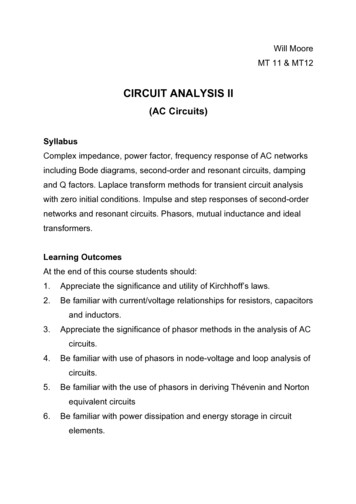
Circuit Analysis II WRM MT119. Phasor diagramsAlthough direct calculation is easily carried out using phasors it issometimes useful to use a phasor (Argand) diagram to show therelationships between say a voltage and current phasor graphically. Inthis way it is easy to see their relative amplitudes and phases and hencegain quick insight into how the circuit operates. As a simple exampleconsider the circuit belowSince the current, I, flows through both elements it is sensible to choosethis as the reference phasor. Having made this choice the voltage dropacross the resistor, VR IR , whereas that across the capacitor,Vc I jωC j ωC I . The sum of these voltages must equal V. Thephasor diagram is easily drawn as39
from which it is clear that the voltage lags the current by an angle φ. Theangle φ may be obtained from the diagram as φ tan1(1 ωCR).Let's consider another exampleWe could obtain the relationship between I and V by using theequivalent impedance derived earlier. However we will use a phasordiagram to show the various currents and voltages which appear acrossthe various components. Since the voltage, V, is the same across eacharm it is sensible to choose this as the reference phasor.The relationships areI 2 jωC V V I1 R jωL I1The two phasor diagrams are40andI I1 I 2
Circuit Analysis II WRM MT11or, combining onto a single diagramwhere φ denotes the phase angle between V and I. In the diagramabove I leads V by φ.41
10.Thévenin and Norton equivalent circuitsThe Thévenin and Norton theorems apply equally well in the AC case.Here we replace any arbitrarily complicated circuit containing resistors,capacitors, inductors by a circuit whose behaviour, as far as the outsideworld is concerned, is entirely equivalent.The two choices are the Thévenin equivalentand the Norton equivalentThe methods for determining V, I and Z are identical to those used in theDC case. In general(i)Calculate the open circuit voltage, Voc(ii) Calculate the short circuit current, Isc42
Circuit Analysis II WRM MT11From whichV Voc ,I Isc andZ VocIscWe note, of course that in the absence of dependent sources it is ofteneasier to "set the sources to zero" and simply calculate the terminalimpedance Zab. We emphasise again that when a voltage source is "setto zero" it is replaced by a short circuit whereas when a current source is"set to zero", no current flows, and hence the source is replaced by anopen circuit.Finally we note that the equivalent impedance Z is also frequentlyreferred to as either(i)internal impedanceor(ii) output impedance.43
ExampleFind the Norton and Thévenin equivalents ofNoting that there are no dependent sources it is easiest to calculate Zabdirectly with the voltage source replaced by a short circuit. This is easysince the circuit then reduces to an inductor in parallel with a resistor.ThusZ Z ab j 40.20 16 j 820 j 40We now need to calculate the open circuit voltage between a and b.This is easy since the circuit is essentially a voltage dividerVoc 20505 exp j 10 20 j 4050 exp j 10 22.3 exp j 53.4 5 exp j 63.4 22.3 53.4 VThus the Thévenin equivalent circuit takes the form44
Circuit Analysis II WRM MT11In order to find the Norton equivalent we need to find the current flowingbetween the terminals a and b when they are shorted together. In thiscase the circuit becomesand50 exp j 10 50 exp j 10 I sc 1.25 exp j 80 1.25 80 j 4040 exp j 90and hence the Norton equivalent becomes45
We have elected to find the Norton equivalent directly. However it isequally possible to transform between Thévenin and Norton equivalentsdirectly as we did in the DC case. It is left as an exercise to confirm thatHence we could have worked out the Norton current source in ourexample directly from the Thévenin equivalent asVoc 22.36 exp j 53.04 I Z16 j 822.36 exp j 53.4 1.25 exp j 80 1.25 80 17.89 exp j 26.6which, of course, is the value we previously calculated.46
Circuit Analysis II WRM MT11 11 3. Circuit analysis with sinusoids Let us begin by considering the following circuit and try to find an expression for the current, i, after the switch is closed. The Kirchhoff voltage law permits us to write Ri V t dt di L m cosω This is a linear differential equation, which you know how to solve.