Transcription
Laboratory ManualELEN 474: VLSI Circuit DesignDepartment of Electrical EngineeringTexas A&M UniversityPrepared by:John S. Mincey (2008)Terry L. Mayhugh, Jr. (1996,1997)Antonio F Mondragon (1998)Dr. Jose Silva-MartinezDr. Jose Pineda de GyvezFall 2009
Table of ContentsLab 0: Introduction . 1Lab 1: Introduction to Cadence. 3Lab 2: Layout Design. 18Lab 3: More Layout Techniques . 28Lab 4: MOS Device Characterization . 31Lab 5: Current Mirrors . 37Lab 6: Inverting Amplifiers . 43Lab 7: Differential Pairs. 54Lab 8: Operational Transconductance Amplifiers . 64Lab 9: 2 Stage Miller OTA . 70i
Lab 0: IntroductionThis laboratory complements the course ELEN 474: VLSI Circuit Design. The labmanual details basic CMOS analog integrated Circuit design, simulation, and testingtechniques. Several tools from the Cadence Development System have been integratedinto the lab to teach students the idea of computer aided design (CAD) and to make theanalog VLSI experience more practical.To fully appreciate the material in this lab course, the student should have aminimal background with the following computer systems, equipment, and circuitanalysis techniques. Students should be familiar with the UNIX operating system.Previous experience using a SPICE-like circuit simulator is also important. This coursedoes not explain the various SPICE analyses and assumes the student is capable ofconfiguring the appropriate SPICE analysis to obtain the desired information from thecircuit. Finally, the student should have general familiarity with active circuit “hand”analysis. All of these prerequisites are satisfied by having credit for ELEN 325 andELEN 326.The lab manual develops the concepts of analog integrated circuit design in abottom-up approach. First, the basic devices of CMOS circuit design, the NMOS andPMOS transistors, are introduced and characterized. Then, one or more transistors arecombined into a subcircuit such as a differential pair, current-mirror, or simple inverterand these small circuits are analyzed. Finally, these subcircuits are connected to formlarger circuits such as operational transconductance amplifiers and operational amplifiers,and the idea of design methodologies is developed. Continuing with the bottom-upapproach, these circuits can be combined to form systems such as filters or dataconverters (not currently covered in this course). The following figure illustrates thebottom-up approach used in the lPairInverterN-MOSTP-MOSTFigure 0-1: Bottom-Up Approach1
The lab activities will generally be one week labs. However there will be somelonger labs toward the end that will be two week labs. Before the lab, the student shouldread through the lab description and perform the pre-lab exercises. Generally, the pre-labexercises are the “hand” design for the circuit being studied. During the lab students willperform circuit simulations to verify their hand calculations. Tweaking circuitparameters will usually need to be done since hand calculations will not always be 100 %accurate. Also, the integrated circuit layout will be created. This will often require moretime to do than 3 hour lab time that is allocated and will need to be finished outside of labsometime before the next lab meeting.Lab ReportEach team will submit one lab report for each lab. Reports are due at thebeginning of class. Lab reports will consist of not more than three typed pages of singlespaced text. Be concise. TITLE PAGE DESCRIPTIONInclude three or four sentences which describe the significant aspects of the lab.This section specifies problems or theory that will be investigated or solved. Thedescription is a more detailed version of the objective. DESIGNInclude circuit diagrams and design formulas/calculations. All circuit diagramsmust be descriptively titled and labeled. A design formula/calculation must begiven for each component. Do not derive equations. RESULTSThis section usually consists of tables and SPICE plots. DISCUSSIONThis is the most important part of the lab report. Simply justify the differencebetween the theoretical and simulated values and answer and needed questions. CONCLUSIONTwo or three sentence summary of what the lab demonstrated. The conclusionusually responds to the problems specified in the DESCRIPTION section.2
Lab 1: Introduction to CadenceObjectivesLearn how to login on a UNIX station, perform basic UNIX tasks, and use theCadence design system to simulate and layout simple circuits.IntroductionThis lab will introduce students to the computer system and software usedthroughout the lab course. First, students will learn how to login and logout of a SunSparcStation. Next, basic operating system commands used to perform file management,printing, and various other tasks will be illustrated. Finally, students will be given anoverview of the Cadence Development System.In-class examples will demonstrate the creation of libraries, the construction ofschematic symbols, the drafting of schematics, and the layout of simple transistors. Thestudent will apply this knowledge to the creation of a CMOS inverter.Logging-In/Logging-OutIn order to use the UNIX machines, you must first login to the system. As withthe PC lab, enter the logon id and password at the prompts. Login using the logon ID andpassword obtained from the electrical engineering office. This is your account and allfiles stored in this area will be retained by the system after logging-out. Do not insert afloppy disk in the SparcStation. There is no need to attempt to make floppy disk backups of your data files.Using the UNIX Operating SystemUsing the UNIX operating system is similar to using other operating systems suchas DOS. UNIX commands are issued to the system by typing them in a “shell” or“xterm”. UNIX commands are case sensitive so be careful when issuing a command,usually they are given in lower-case.The following list summarizes all the basic commands required to manage thedata files you will be creating in this lab course. All UNIX commands are entered fromthe shell or xterm window. Do not use UNIX commands for modifying, deleting, ormoving any Cadence data files.3
Table 1-1: Common UNIX Commandsls [–la]Lists files in the current directory. ”l” lists with properties and“a” also lists hidden files (ones beginning with a “.”).cd XXXXChanges the current directory to XXXX.cd .Changes the current directory back one level.cp XXXX YYYYCopies the file XXXX to YYYY.mv XXXX YYYYMove file XXXX to YYYY. Also used for renamerm XXXXDeletes the file XXXXmkdir XXXXCreates the directory XXXX.lp -dXXXX YYYYPrints the textfile or postscript file YYYY to the printer namedXXXX, where XXXX can be either “ipszac” or “hpszac”.gedit XXXX&Starts the gedit text editor program and loads file XXXX.icfb &Starts the Cadence software.topCheck available processes and memory usage.quota –vCheck for disk space availablewho grep my nameDisplay the terminal where I am connectedNote: The command “&” tells UNIX to execute the command and return the prompt tothe active shell.CadenceThe Cadence Development System consists of a bundle of software packagessuch as schematic editors, simulators, and layout editors. This software manages thedevelopment process for analog, digital, and mixed-mode circuits. In this course, we willstrictly use the tools associated with analog circuit design.All the Cadence design tools are managed by a software package called theDesign Framework II. This program supervises a common database which holds allcircuit information including schematics, layouts, and simulation data.From the Design Framework II also known as the "framework", we can invoke aprogram called the Library Manager which governs the storage of circuit data. We canaccess libraries and the components of the libraries called cells.Also, from the framework we can invoke the schematic entry editor called"Composer". Composer is used to draw circuit diagrams and draw circuit symbols.A program called "Virtuoso" is used for creating integrated circuit layouts. Thelayout is used to create the masks which are used in the integrated circuit fabricationprocess.Finally, circuit simulation is handled through an interface called "Analog Artist."This interface can be used to invoke various simulators including HSPICE, Spectre, andVerilog. We will be using the SpectreS simulator in this course.4
Starting Cadence for the First TimeAll Cadence simulations need to be run on the Sunfire server. To connect to this server,you should type the following commands into a terminal:ssh –X sunfire.ece.tamu.eduDO NOT CLOSE THE TERMINAL. It must remain open the whole time you haveCadence running.Before Cadence can be run, some basic configuration of your system needs to be done.We need to first edit our .cshrc file so that the correct version of cadence is run. You cando this with any text editor that you wish. If you are new to UNIX, I recommend aprogram called “gedit” since it is very similar to Notepad in Windows. From a terminaltype:cdgedit .cshrc &In the text editor that opens, you need to add the following two lines to the end of the file:source /usr/local/bin/setup.ic5141setenv CDK DIR /baby/cadence/ic50/localSave the changes you made to .cshrc and close the file. At the terminal type:source .cshrcNext, edit your .cdsenv file.cdgedit .cdsenvAdd the line:asimenv.startup cds ade wftool string “awd”Next we need to make a new directory called “cadence” which will hold all of ourcadence files. This will also be the directory you need to run Cadence from in the future.In this folder we will also put two more configuration files, cds.lib and .cdsinit.mkdir cadencecd cadencecp /baby/courses/474/cds.lib /cadencecp /baby/courses/474/.cdsinit /cadenceCadence should be ready to run now. From now on, you can launch Cadence when youlogin to Sunfire by typingcd cadenceicfb &This will load Cadence. The Command Interpreter Window (CIW) will now load asshown in Figure 1-1.5
Figure 1-1: The Cadence CIWStarting a DesignFrom the CIW select Tools Library Manager to load the Library Manager(Figure 1-2). The Library Manager stores all designs in a hierarchal manner. A library isa collection of cells. For example, if you had a digital circuits library named Digital, itwill have several cells included in it. These cells will be inverters, nand gates, nor gates,multiplexers, etc. Each cell has different views. These views will in general be thingssuch as symbols, schematics, or layouts of each cell.Figure 1-2: Library ManagerThe first thing you need to do to start a design is create a library to store the cellsyou will be designing in this lab. Let’s call this library “ee474”. From the LibraryManager select File New Library. Name the library “ee474” (without quotes) andselect OK. In the window that appears select “Attach to an existing techfile” (Figure 1-3)and select OK. In the next window (Figure 1-4) make sure that NCSU TechLib ami06is selected and select OK.6
Figure 1-3: Attach to an existing techfileFigure 1-4: Attaching to a library to a technology fileCreating a SchematicThe first circuit we will design is a simple inverter. Select which library you wantto put the cell into, in this case “ee474”, and then File New Cell. Name your cellinverter. The tool you want to use here is Composer-Schematic as seen in Figure 1-5.Figure 1-5: Creating a new cell view7
After selecting OK, the schematic window opens. We wish to add two transistorsso that we can make an inverter. To do this we need to add an instance. You can do thisby either clicking Add Instance or by pressing “i” on the keyboard. A window titled“Component Browser” should pop up. Make sure that the library NCSU Analog Parts isselected. Select N Transistors and then nmos4. Go back to the schematic and selectwhere you would like to add the NMOS transistor. Go back to the Component Browserand select P transistors and then pmos4. Add this transistor to your schematic. Hit ESCto exit the Add Instance mode.Connect components together using wires. You can select Add Wire or usethe “w” hotkey.Pins identify the inputs and outputs of the schematic. Click Add Pin or use the“p” hotkey. Pin names and directions must be consistent between the symbol, schematic,and layout. The name uniquely identifies the pin while the direction indicates the usageof the pin. I recommend using the inputOutput direction for all pins.To change the properties of a device use Edit Properties Objects or use the“q” hotkey. Try changing the width of the PMOS transistor from 1.5u to 3u. Whenfinished, your schematic should resemble Figure 1-6.Figure 1-6: InverterSelect Design Check and Save to save your schematic and make sure that thereare no errors or warnings.Creating a SymbolWithout closing the schematic window select Design Create Cellview FromCellview. Make sure that “schematic” is selected in the “From View Name” field. Tool /Data Type needs to be “symbol”. Select OK and then OK again on the next window.8
Figure 1-7: Create cellview from cellviewThe symbol created should resemble the one in Figure 1-8. This does notresemble an inverter symbol at all. We can redraw it by deleting some lines and addingnew ones. The final symbol should resemble Figure 1-9.Figure 1-8: Default SymbolFigure 1-9: Final Inverter Symbol9
Creating a LayoutAfter the schematic and symbol have been designed, it is time to move onto thelayout of the circuit. From the library manager select File New Cell View. Layoutis done using the tool named Virtuoso. Select Virtuoso as the toolname (Figure 1-10).After clicking OK, Virtuoso should open as well as the layer selection window (LSW,Figure 1-11).The layout consists of rectangles, instances, and pins. A rectangle is used tocreate gate, diffusion, and metal regions for the transistor. The gate region is created bydrawing a rectangle with poly (drw). The diffusions for a transistor are created bydrawing a rectangle with the active (drw) layer. The intersection of poly and activeregions defines the size (length and width) of the transistors. In order to define whether aFigure 1-10: Creating a layout cell view10
Figure 1-11: The LSW11
transistor is NMOS or PMOS, nselect (drw) or pselect (drw) needs to surround the activearea. The design rules describe minimum spacing and size requirements for variousrectangles. Some basic design rules for this technology are shown in Figure 1-12.Figure 1-12: Basic design rulesSubstrate contacts and vias between layers of metal can be drawn by hand, beadded by selecting Create Contact, or by using the “o” hotkey.To add a pin, select Create Pin. “Terminal Name” should be the name of thepin in the schematic. Make sure that the “Display Pin Name” option is selected so thatthe pin name will appear in the layout. “Pin Type” should be the same as the metal layerthat it is connecting to.After completing the above steps, you should obtain a layout of the inverter whichresembles Figure 1-13.After the layout is done, several steps have to be followed to insure that the layoutis correct. These steps involve performing the following analysis:Table 1-2: Post layout stepsDRCDesign Rule Check. Checks physical layout data against fabrication-specificrules. Typical checks include spacing, enclosure and overlap.Extract Device parameter and connectivity are extracted from the layout in order toperform ERC, Short Locator, LVS and post-layout simulation and analysis.LVSLayout Versus Schematic. Compares a physical layout design to the schematicfrom where it was designed.12
Figure 1-13: Inverter layoutDRCTo run DRC for the layout, select Verify DRC. You do not need to make anymodifications to the window that opens up. Select OK to run the DRC. The total numberof errors will show up in the CIW as seen in Figure 1-14. Before going further we haveto reduce the number of errors to 0.Figure 1-14: CIW showing DRC errorsThe errors will usually show up in the layout as white lines. To have Cadenceexplain what the error is, select Verify Markers Explain. Click on one of the whitelines, and Cadence will explain what design rule you broke. Adjust the layout to fix theseerrors and then rerun DRC until you have no design rule errors.13
ExtractOnce DRC is completed, you can now extract the layout. Select Verify Extract. From this window, select “Set Switches”. Highlight “Extract Parasitic Caps”and then click OK. Click OK again to extract the layout to make the extracted netlist.LVSThe LVS window is shown in Figure 1-15. Make sure Rewiring, Device Fixing,and Terminals are selected under LVS Options. Click Run. A window should pop uponce LVS has completed saying that the job succeeded. Click OK. From the LVSwindow select output. The output should have a line that says “The net-lists match.” Ifthey do not match, go back to the LVS window. Select Error Display to find out whatyour errors are. Adjust the layout to match, rerun DRC, Extract, and LVS until thenetlists match.Once the schematic and layout match, go back to the LVS window and clickBuild Analog and then OK.Figure 1-15: LVS window14
Simulating the SchematicTo test the inverter, we need to create a new schematic cell view called“inverter test”. To simulate the design, add the inverter symbol, signal sources, powersupplies, and loads as illustrated in Figure 1-16.Figure 1-16: Inverter test schematicStart the simulator environment by selecting Tools Analog Environment. Thesimulator should appear in a few moments. Select Setup Simulator/Directory/Hostand verify that spectreS is the simulator.Next we need to configure the environment to run our first simulation. In theAnalog Environment window select Analyses Choose. Select “dc” and then“Component Parameter”. Select “Select Component” and then click on the desiredvoltage source in the schematic to sweep. In this case we want to sweep the input voltagesource which is V0 in Figure 1-16. Select “dc” as the variable to sweep when the popupwindow opens. We wish to sweep the source from the negative supply to the positivesupply, so input -1.5 into “Start” and 1.5 into “Stop”. Select OK.The simulator should now be configured to run the simulation. Select Simulation Run or click on the green light in the bottom right corner. Once the simulation hascompleted, we can plot any outputs that we wish. To do this we use the calculator. Toaccess the calculator, select Tools Calculator in the Analog Environment.Since our analysis that was ran was a dc sweep, click the “vs” button (The “v” isfor voltage and the “s” is for DC sweep.) Next click on the output node in the schematic.You can now plot the output as a function of the swept variable, which in this case is theinverter input, by clicking “plot”. Your output waveform should resemble Figure 1-17.15
Figure 1-17: Inverter output plotSimulating the Extracted LayoutTo simulate the layout to verify that it operates as desired, you must do one thingin the Analog Environment before running simulations. You will still open the AnalogEnvironment through the schematic window.In the Analog Environment, select Setup Environment. In the field labeled“Switch View List” add “analog exracted” before “schematic” as shown in Figure 1-18.All other steps in simulation of the extracted view will now be the same as they were forsimulating the schematic.16
Figure 1-18: Adding extracted view to switch view listPrelabThis prelab exercise is to be done during the lab under supervision of the TA.Turn in print outs of the following with the lab report next week:1) Inverter schematic2) Inverter symbol3) DC sweep output graph showing the inverter was simulated4) Inverter layout5) Copy of the LVS output file showing that the netlists matchLab ReportNo lab report is required this week other than the printouts listed in the Prelabsection.17
Lab 2: Layout DesignObjectiveLearn techniques for successful integrated circuit layout design.IntroductionIn this lab you will learn in detail how to generate a simple transistor layout.Next, techniques will be developed for generating optimal layouts of wide transistors andmatched transistors. Layout techniques for resistors and capacitors will also beillustrated. Finally, you will use all of these layout techniques to produce a two-stageopamp layout (Lab 3).Layout TechniquesTransistorsIn Lab 1 you learned how to layout small size transistors. Most analog designswill not be limited to these small width transistors, thus special layout techniques need tobe learned to layout large width MOSFETS. Luckily, wide transistors can be broken intoparallel combinations of small width transistors as seen in Figure 2-1. By doing thishorizontal expansion technique for the wide transistor, the drain and source area can bereduced which decreases parasitic capacitance and resistance.Figure 2-1: Wide MOS transistor layoutAnother good layout technique is to use “dummy” transistors on both ends of atransistor layout. These dummy transistors insure that the etching and diffusionprocesses occur equally over all segments of the transistor layout.18
Figure 2-2: Dummy transistor layoutNotice the gate, drain, and source are connected together which keeps it fromconducting any current. This shorted transistor is connected to the drain or source of thefunctional transistor. Another alternative for dummy transistors is to have the gate andsource tied together.When laying out any device the key is symmetry, especially when laying outfully-differential components. For matched devices, use interdigitized or commoncentroid layout techniques. A matched device is one where two transistors need to haveexactly the same geometries. Examples include current mirrors and differential pairs.An interdigitized layout is shown in Figure 2-3. Notice that the two transistorshave been split into smaller size devices and interleaved. This layout minimizes theeffects of process variations on the parameters of the transistors.The idea behind splitting a transistor up is to average the process parametergradient over the area of the matched devices. For example, the process variation of KPand of the transconductance parameter on the wafer is characterized by a global variationand a local variation. Global variations appear as gradients on the wafer as in Figure 2-4.However, local variations describe the random change in the parameter from one point onthe chip to another nearby point. By using layout techniques such as interdigitized andcommon-centroid, the process variation can hopefully be averaged out among thematched devices.When laying out wider matched transistors the common-centroid layout may be abetter choice. This layout technique is illustrated in Figure 2-5 for the case of 8 matchedM1 and M2 transistors of a differential pair.19
SD2SD1SD2SSD2G1d)Figure 2-3: Interdigitized layout of a differential paira) Differential pairb) Horizontal expansionc) Interdigitized layout (Drain areas are different. Common centroid.)d) Interdigitized layout (Drain areas are equal. Not common centroid.)KP 27 A V 2KP 20 A V 2KP 29 A V 2KP 25 A V 2KP 33 A V 220
Figure 2-4: Gradient of KP on a waferG2D1D1SD2SD1SD2SD1SD2G1D2SD1SD2SD1SD2SFigure 2-5: Common-centroid layout of a differential pairThe idea behind the common-centroid layout is to average linear processinggradients that affect the transistors’ electrical properties. Common-centroid layoutsshould have the centroid (center of mass) of each transistor positioned at the samelocation. The following examples illustrate what is common-centroid and what is notcommon-centroid.21
Figure 2-6: Common-centroid examplesCapacitorsCapacitors of various types can be fabricated on integrated circuits. A capacitor isformed when an insulator separates two conducting sheets. Two methods of formingcapacitors are by using poly and poly2 (elec layer in LSW) as the capacitor iainstancem1 elecinstancenwcinstancem1 ectangleelecFigure 2-7: Poly-Poly2 capacitor layoutFigure 2-7 illustrates the layout of the poly-poly2 capacitor. The capacitor isformed by laying a second layer of polysilicon over the gate polysilicon. The area of thetop plate (poly2) and the perimeter determine the capacitance by the following equation:C CA A CF Pwhere:CAis the capacitance per unit area for the chosen capacitor typeAis the area of the top capacitor plateCFis the fringe capacitance per unit length for the chosen capacitor type fordiffusion based capacitorsPis the perimeter of the top capacitor plate22
For poly-poly2 capacitors, a parasitic capacitance between the substrate and polycan inject unwanted signals and noise into the circuit at the bottom plate of the capacitor.To reduce this problem, put the capacitor in an N-well (for an N-well process) andconnect the well to a “clean” ground. A ground plane (metal sheet connected to ground)can be used as a shield by covering all capacitors where possible.For poly-diffusion capacitors, the bottom plate is placed in a special capacitorwell to reduce noise injection and to prevent voltage signals from altering thecapacitance. This produces a high quality linear capacitance.To prevent the injection of noise from the substrate into the bottom plate of thecapacitor, always be sure to connect it to a low impedance node such as ground or theoutput of an op-amp. Do not connect the bottom plate of a capacitor to an op-amp input.The substrate noise is due partly to power supply noise and connecting the bottom plateto the op-amp input allows direct injection of power supply noise into the op-amp input.The power supply is used to bias the substrate, so they are usually directly connected.When designing circuits, sometimes desired circuit performance depends on theratio of two capacitors. In such cases, it is important that two are more capacitors areproperly matched. Divide each capacitor into many smaller “unit” capacitors. Formatched devices this keeps the ratio of the areas and the ratios of the perimeters the same.Like matched MOSFETS, the common-centroid layout technique can beemployed for matched capacitors. Figure 2-8 gives a simplified layout floor plan for twoequally sized, well-matched capacitors.Figure 2-8: Common-centroid capacitor layoutThe absolute and matching accuracy for various types of capacitors is given in thefollowing table:CapacitorAbsolute AccuracyMatching AccuracyPoly1-Poly2Poly-Diffusion 20% 10% 0.06% 0.06%23
Remember, the purpose of using the unit capacitor is to keep the ratio of the areasand perimeters the same. This prevents (delta) variations in capacitor dimensions fromchanging the capacitor ratio. If a non-integral number of unit capacitors are required, thenthe perimeters and areas can still be kept the same. If the ratio of capacitors isC1 I N , where 1 N 2, then the unit capacitor has side length L0 and the non-unitC2capacitor has side lengths L1 and L2. Use the following formulas to calculate the sidelengths of the non-unit capacitor: L1 L0 N N N 1 20LL1Keep the unit capacitor side length L0 in the range from 10 m-25 m. Also,within the capacitor array, use a consistent method of routing lines between the capacitorsegments. Each unit capacitor should be surrounded by similar routing lines. Forcapacitors near the edge of the array, use “dummy” routing lines. Also, be sure thatparasitic capacitance formed by overlapping conductors is the same for the matchedcapacitors.L2 NLarge unmatched capacitors can be divided into smaller unit capacitors to reducedistributed effects caused by the relatively high resistivity polysilicon. This prevents alarge capacitor which possesses considerable resistivity as well as capacitance fromacting as a lossy transmission line.ResistorsAs for capacitors, many different types of resistors are available in integratedcircuits. Other than active devices biased to act as resistors, we can use the inherentresistivity of the polysilicon or diffusions to create resistors. The following table showsthe typical values of resistance for the AMI 0.5μm process that we will be using to designcircuits.PROCESS PARAMETERSM1M2UNITSSheet Resistance0.09 0.09 ohms/sqContact Resistance0.90 ohmsN P POLY83.9109.522.364.7169.615.6PLY2 HRPOLY2101440.325.9The total resistance of a monolithic resistor is the sum of the contact resistanceand the ohmic resistance of the diffusion material. The following formula can be used toestimate resistance for polysilicon and diffusion resistors:R RS L 2 RCW24
where:RSis the resistance per square for the chosen resistor typeLis the length of the resistorWis the width of the transistorRCis the contact resistanceFigure 2-9 shows a polysilicon resistor layout. The resistor is constructing byadding a strip of poly and then by adding poly contacts. Next the “res id” layer is addedwhich tells the extraction program that this is a resistor that needs
circuit. Finally, the student should have general familiarity with active circuit "hand" analysis. All of these prerequisites are satisfied by having credit for ELEN 325 and ELEN 326. The lab manual develops the concepts of analog integrated circuit design in a bottom-up approach. First, the basic devices of CMOS circuit design, the NMOS and