![[scale 0.25]FIG/bande-n7-tete.pdf *.75cm Sparse Linear . - ENSEEIHT](/img/30/alc-toulouse.jpg)
Transcription
Sparse Linear Algebra: Direct Methods, advanced featuresP. Amestoy and A. Buttari(INPT(ENSEEIHT)-IRIT)A. Guermouche (Univ. Bordeaux-LaBRI),J.-Y. L’Excellent and B. Uçar (INRIA-CNRS/LIP-ENS Lyon)F.-H. Rouet (Lawrence Berkeley National Laboratory)C. Weisbecker INPT(ENSEEIHT)-IRIT2013-2014
Sparse Matrix Factorizations A m m , symmetric positive definite LLT AAx b A m m , symmetric LDLT AAx b A m m , unsymmetric LU AAx b A m n ,m 6 n QR Amin kAx bkxmin kxk such thatif m nAx b if n m
Cholesky on a dense matrix a11 a21 a22 a31 a32 a33 a41 a42 a43 a44Left lookingRight lookingused for modificationmodifiedleft-looking Choleskyfor k 1, ., n dofor i k, ., n dofor j 1, ., k 1 do(k)(k)aik aik lij lkjend forend forq(k 1)lkk akkfor i k 1, ., n do(k 1)/lkklik aikend forend forright-looking Choleskyfor k 1,q., n do(k 1)lkk akkfor i k 1, ., n do(k 1)lik aik/lkkfor j k 1, ., i do(k)(k)aij aij lik ljkend forend forend for
138JOSEPH W. H. LIUFactorization of sparse matrices: problemsThe factorization of a sparse matrix is problematic due to thepresence of fill-in.aThe basic LU step:(k) (k)(k 1)JOSEPHW. H. LIU ai,j138(k)(k 1)Even if ai,j is null, ai,j(k)ai,j dai,k ak,j(k)ak,kcan be a nonzerofaaoddIooh0ofaoo the factorization is more expensive than O(nz)FIG. 2.1. An example of matrix structures.o higher amountof memory requiredthan O(nz)d more complicated algorithms to achieve the factorizationI
Factorization of sparse matrices: problemsBecause of the fill-in, the matrix factorization is commonly precededby an analysis phase where: the fill-in is reduced through matrix permutations the fill-in is predicted though the use of (e.g.) elimination graphs computations are structured using elimination treesThe analysis must complete much faster than the actual factorization
Analysis
Fill-reducing ordering methodsThree main classes of methods for minimizing fill-in duringfactorizationLocal approaches : At each step of the factorization, selection of thepivot that is likely to minimize fill-in. Method is characterized by the way pivots areselected. Markowitz criterion (for a general matrix) Minimum degree (for symmetric matrices)Global approaches : The matrix is permuted so as to confine thefill-in within certain parts of the permuted matrix Cuthill-McKee, Reverse Cuthill-McKee Nested dissectionHybrid approaches : First permute the matrix globally to confine thefill-in, then reorder small parts using local heuristics.
The elimination process in the graphsGU (V, E) undirected graph of Afor k 1 : n 1 doV V {k} {remove vertex k}E E {(k, ) : adj(k)} {(x, y) : x adj(k) and y adj(k)}Gk (V, E) {for definition}end forGk are the so-called elimination graphs (Parter,’61).214G0 :613H0 523456
The Elimination TreeThe elimination tree is a graph that expresses all the dependencies inthe factorization in a compact way.Elimination tree: basic138 ideaJOSEPH W. H. LIUIf i depends on j (i.e., lij 6 0, i j) and k depends on i (i.e.,lki 6 0, k i), then k depends on j for the transitive relation andtherefore, the direct dependency expressedby lkj 6 0, if it exists, isaredundantdFor each JOSEPHcolumnj n of L, remove all the nonzeros in the column jW. H. LIUexcept the first one below the diagonal.Let Lt denote the remaining structure and consider the matrixFt Lt LTt . The graph G(Ft ) is a tree called the elimination tree.faaoddIooh0ooooj
Uses of the elimination treeThe elimination tree has several uses in the factorization of a sparsematrix: it expresses the order in which variables can be eliminated: the elimination of a variable only affects (directly or indirectly) itsancestors and . . only depends on its descendantsTherefore, any topological order of the elimination tree leads to acorrect result and to the same fill-in it expresses concurrence: because variables in separate subtrees donot affect each other, they can be eliminated in parallel
Matrix factorization
Cholesky on a sparse matrixThe Cholesky factorization of a sparse matrix can be achieved with aleft-looking, right-looking or multifrontal method.Reference case: regular 3 3 grid ordered by nested dissection.Nodes in the separators are ordered last (see the section on orderings)91748738632965124Notation: cdiv(j):ppA(j, j) and then A(j 1 : n, j)/ A(j, j) cmod(j,k): A(j : n, j) A(j, k) A(j : n, k) struct(L(1:k,j)): the structure of L(1:k,j) submatrix5
Sparse left-looking Cholesky9left-lookingfor j 1 to n dofor k in struct(L(j,i:j-1)) docmod(j,k)end forcdiv(j)end for8731624In the left-looking method, before variable j is eliminated, column j isupdated with all the columns that have a nonzero on line j. In theexample above, struct(L(7,1:6)) {1, 3, 4, 6}. this corresponds to receiving updates from nodes lower in thesubtree rooted at j the filled graph is necessary to determine the structure of each row5
Sparse right-looking Cholesky9right-lookingfor k 1 to n docdiv(k)for j in struct(L(k 1:n,k)) docmod(j,k)end forend for8731624In the right-looking method, after variable k is eliminated, column kis used to update all the columns corresponding to nonzeros incolumn k. In the example above, struct(L(4:9,3)) {7, 8, 9}. this corresponds to sending updates to nodes higher in theelimination tree the filled graph is necessary to determine the structure of eachcolumn5
The Multifrontal MethodEach node of the elimination tree is associated with a dense frontThe tree is traversed bottom-up and at each node1. assembly of the front2. partial factorization9867897316245467569
The Multifrontal MethodEach node of the elimination tree is associated with a dense frontThe tree is traversed bottom-up and at each node1. assembly of the front2. partial factorization986789731 a44 a64a74a46006244675 a47l44 0 l640l74 b66b76b67 b77569
The Multifrontal MethodEach node of the elimination tree is associated with a dense frontThe tree is traversed bottom-up and at each node1. assembly of the front2. partial factorization986789731 a55 a65a95a56006244675 a59l55 0 l650l95 c66c96c69 c99569
The Multifrontal MethodEach node of the elimination tree is associated with a dense frontThe tree is traversed bottom-up and at each node1. assembly of the front2. partial factorization986789731 a66 0 a8600000a68000624 0b66 b67 0 0 b76 b77 00 0000000 l66 l76 d77 d78 l86 d87 d88l86 d97 d984675 0c66 0 00 00c96 d79 d89 d9956900000000 c690 0 c99
The Multifrontal MethodA dense matrix, called frontal matrix, is associated at each node ofthe elimination tree. The Multifrontal method consists in a bottom-uptraversal of the tree where at each node two operations are done: Assembly Nonzeros from the original matrix are assembledtogether with the contribution blocks from children nodes into thefrontal matrixarrowhead cb-1cb-n . Elimination A partial factorization of the frontal matrix is done.The variable associated to the node of the frontal tree (called fullyassembled) can be eliminated. This step produces part of the finalfactors and a Schur complement (contribution block) that will beassembled into the father nodeLfrontalmatrixcb
The Multifrontal Method: example654312
Solve
SolveOnce the matrix is factorized, the problem can be solved against oneor more right-hand sides:AX LLT X B,A, L Rn n ,X Rn k ,B Rn kThe solution of this problem can be achieved in two steps:forward substitution LZ Bbackward substitution LT X Z
Solve: left-lookingForward Substitution987 3162Backward Substitution45987 316245
Solve: right-lookingForward Substitution987 3162Backward Substitution45987 316245
Direct solvers: resumeThe solution of a sparse linear system can be achieved in three phasesthat include at least the following operations:Analysis Fill-reducing permutation Symbolic factorization Elimination tree computationFactorization The actual matrix factorizationSolve Forward substitution Backward substitutionThese phases, especially the analysis, can include many otheroperations. Some of them are presented next.
Parallelism
Parallelization: two levels of parallelismtree parallelism arising from sparsity, it is formalized by the fact thatnodes in separate subtrees of the elimination tree can beeliminated at the same timeDecreasing tree parallelismIncreasing node parallelismnode parallelism within each node: parallel dense LU factorization(BLAS)LUULUL
Exploiting the second level of parallelism is crucialComputerAlliant FX/80IBM 3090J/6VFCRAY-2CRAY Y-MP#procs8646MFlops15126316529Multifrontal factorization(1)(2)(speed-up) MFlops .3)1119(4.8)Performance summary of the multifrontal factorization on matrix BCSSTK15. Incolumn (1), we exploit only parallelism from the tree. In column (2), we combinethe two levels of parallelism.
Task mapping and schedulingTask mapping and scheduling: objectiveOrganize work to achieve a goal like makespan (total execution time)minimization, memory minimization or a mixture of the two: Mapping: where to execute a task? Scheduling: when and where to execute a task? several approaches are possible: static: Build the schedule before the execution and follow it atrun-time Advantage: very efficient since it has a global view of the system Drawback: Requires a very-good performance model for the platform dynamic: Take scheduling decisions dynamically at run-time Advantage: Reactive to the evolution of the platform and easy to useon several platforms Drawback: Decisions taken with local criteria (a decision which seemsto be good at time t can have very bad consequences at time t 1) hybrid: Try to combine the advantages of static and dynamic
Task mapping and schedulingThe mapping/scheduling is commonly guided by a number ofparameters: First of all, a mapping/scheduling which is good for concurrency iscommonly not good in terms of memory consumption181617121112341356147910 Especially in distributed-memory environments, data transfers haveto be limited as much as possible
Dynamic scheduling on shared memory computersThe data can be shared between processors without anycommunication , therefore a dynamic scheduling is relatively simpleto implement and efficient: The dynamic scheduling can be done through a pool of “ready”tasks (a task can be, for example, seen as the assembly andfactorization of a front) as soon as a task becomes ready (i.e., when all the tasksassociated with the child nodes are done), it is queued in the pool processes pick up ready tasks from the pool and execute them. Assoon as one process finishes a task, it goes back to the pool topick up a new one and this continues until all the nodes of the treeare done the difficulty lies in choosing one task among all those in the poolbecause the order can influence both performance and memoryconsumption
Decomposition of the tree into levels Determination of Level L0 based on subtree 7,86 7Subtree roots Scheduling of top of the tree can be dynamic.8
Simplifying the mapping/scheduling problemThe tree commonly contains many more nodes than the availableprocesses.Objective : Find a layer L0 such that subtrees of L0 can be mappedonto the processor with a good balance.Step AStep BStep CConstruction and mapping of the initial level L0Let L0 Roots of the assembly treerepeatFind the node q in L0 whose subtree has largest computationalcostSet L0 (L0 \{q}) {children of q}Greedy mapping of the nodes of L0 onto the processorsEstimate the load unbalanceuntil load unbalance threshold
Static scheduling on distributed memory computersMain objective: reduce the volume of communication betweenprocessors because data is transferred through the (slow) network.Proportional mapping initially assigns all processes to root node. performs a top-down traversal of the tree where the processesassign to a node are subdivided among its children in a way that isproportional to their relative 4614474,545910Mapping of the tasks onto the 5 processorsGood at localizingcommunication but not soeasy if no overlappingbetween processorpartitions at each step.
Assumptions and Notations Assumptions : We assume that each column of L/each node of the tree is assignedto a single processor. Each processor is in charge of computing cdiv(j) for columns j thatit owns. Notation : mycols(p) is the set of columns owned by processor p. map(j) gives the processor owning column j (or task j). procs(L(:,k)) {map(j) — j struct(L(:,k))}(only processors in procs(L(:,k)) require updates from column k –they correspond to ancestors of k in the tree). father(j) is the father of node j in the elimination tree
Computational strategies for parallel direct solversThe parallel algorithm is characterized by: Computational graph dependency Communication graphThere are three classical approaches to distributed memoryparallelism:1. Fan-in : The fan-in algorithm is very similar to the left-lookingapproach and is demand-driven: data required are aggregatedupdate columns computed by sending processor2. Fan-out : The fan-out algorithms is very similar to theright-looking approach and is data driven: data is sent as soon asit is produced.3. Multifrontal : The communication pattern follows a bottom-uptraversal of the tree. Messages are contribution blocks and are sentto the processor mapped on the father node
Fan-in variant (similar to left looking)987316245fan-infor j 1 to nu 0for all k in (struct(L(j,1:j-1)) mycols(p) )cmod(u,k)end forif map(j) ! psend u to processor map(j)elseincorporate u in column jreceive all the updates on column j and incorporate themcdiv(j)end ifend for
Fan-in variantP4P0P1P2P3
Fan-in variantP4P0P1P2P3
Fan-in variantP4P0P1P2P3
Fan-in variantP4P0P1P2P3
Fan-in variantP4P0P1P2P3
Fan-in variantP4CommunicationP0P1P2P3
Fan-in variantP4CommunicationP0P0P0P0if i children map(i) P 0 and map(f ather) 6 P 0 (only) onemessage sent by P 0 exploits data locality of proportional mapping.
Fan-out variant (similar to right-looking)98731fan-outfor all leaf nodes j in mycols(p)cdiv(j)send column L(:,j) to procs(L(:,j))mycols(p) mycols(p) - {j}end forwhile mycols(p) ! receive any column (say L(:,k))for j in struct(L(:,k)) mycols(p)cmod(j,k)if column j is completely updatedcdiv(j)send column L(:,j) to procs(L(:,j))mycols(p) mycols(p) - {j}end ifend forend while6245
Fan-out variantP4P0P1P2P3
Fan-out variantP4CommunicationP0P0P0P0if i children map(i) P 0 and map(f ather) 6 P 0 then nmessages (where n is the number of children) are sent by P 0 toupdate the processor in charge of the father
Fan-out variantP4CommunicationP0P0P0P0if i children map(i) P 0 and map(f ather) 6 P 0 then nmessages (where n is the number of children) are sent by P 0 toupdate the processor in charge of the father
Fan-out variantP4CommunicationP0P0P0P0if i children map(i) P 0 and map(f ather) 6 P 0 then nmessages (where n is the number of children) are sent by P 0 toupdate the processor in charge of the father
Fan-out variantP4CommunicationP0P0P0P0if i children map(i) P 0 and map(f ather) 6 P 0 then nmessages (where n is the number of children) are sent by P 0 toupdate the processor in charge of the father
Fan-out variantProperties of fan-out: Historically the first implemented. Incurs greater interprocessor communications than fan-in (ormultifrontal) approach both in terms of total number of messages total volume Does not exploit data locality of proportional mapping. Improved algorithm (local aggregation): send aggregated update columns instead of individual factor columnsfor columns mapped on a single processor. Improve exploitation of data locality of proportional mapping. But memory increase to store aggregates can be critical (as in fan-in).
Multifrontal98731624multifrontalfor all leaf nodes j in mycols(p)assemble front jpartially factorize front jsend the schur complement to procs(father(j))mycols(p) mycols(p) - {j}end forwhile mycols(p) ! receive any contribution block (say for node j)assemble contribution block into front jif front j is completely assembledpartially factorize front jsend the schur complement to procs(father(j))mycols(p) mycols(p) - {j}end ifend while5
Multifrontal rontal
Multifrontal rontal
Multifrontal rontal
Multifrontal rontal
Multifrontal rontal
Importance of the shape of the treeSuppose that each node in the tree corresponds to a task that: consumes temporary data from the children, produces temporary data, that is passed to the parent node. Wide tree Good parallelism Many temporary blocks to store Large memory usage Deep tree Less parallelism Smaller memory usage
Impact of fill reduction on the shape of the treeReorderingtechniqueAMDShape of the treeobservations Deep well-balanced Large frontal matrices ontopAMF Very deep unbalanced Small frontal matrices
Impact of fill reduction on the shape of the treePORD deep unbalanced Small frontal matricesSCOTCH Very wide well-balanced Large frontal matricesMETIS Wide well-balanced Smaller frontal matrices(than SCOTCH)
Memory consumption in the multifrontal method
Equivalent reorderingsA tree can be regarded as dependency graph where node producedata that is, then, processed by its parent.By this definition, a tree has to be traversed in topological order. Butthere are still many topological traversals of the same tree.DefinitionTwo orderings P and Q are equivalent if the structures of the filledgraphs of P AP T and QAQT are the same (that is they areisomorphic).Equivalent orderings result in the same amount of fill-in andcomputation during factorization. To ease the notation, we discussonly one ordering wrt A, i.e., P is an equivalent ordering of A if thefilled graph of A and that of P AP T are isomorphic.
Equivalent reorderingsAny topological ordering on T (A) are equivalentLet P be the permutation matrix corresponding to a topologicalordering of T (A). Then, G (P AP T ) and G (A) are isomorphic.Any topological ordering on T (A) are equivalentLet P be the permutation matrix corresponding to a topologicalordering of T (A). The elimination tree T (P AP T ) and T (A) areisomorphic.Because the fill-in won’t change, we have the freedom to choose anyspecific topological order that will provide other properties
Tree traversal ordersWhich specific topological order to choose? postorder: why?Because data produced by nodes is consumed by parents in a LIFOorder.In the multifrontal method, we can thus use a stack memory wherecontribution blocks are pushed as soon as they are produced by theelimination on a frontal matrix and popped at the moment where thefather node is assembled.This provides a better data locality and makes the memorymanagement easier.
The multifrontal method [Duff & Reid ’83]512A 3451 2 3 4 512L U-I 3451 2 3 4 5Storage is divided into two parts: Factors Active memoryFactorsActive Stack offrontal contributionmatrix blocksActive storage451453423Elimination tree
The multifrontal method [Duff & Reid ’83]512A 3451 2 3 4 512L U-I 3451 2 3 4 5Storage is divided into two parts: Factors Active memory451453423Active memory
The multifrontal method [Duff & Reid ’83]512A 3451 2 3 4 512L U-I 3451 2 3 4 5Storage is divided into two parts: Factors Active memory451453423Active memory
The multifrontal method [Duff & Reid ’83]512A 3451 2 3 4 512L U-I 3451 2 3 4 5Storage is divided into two parts: Factors Active memory451453423Active memory
The multifrontal method [Duff & Reid ’83]512A 3451 2 3 4 512L U-I 3451 2 3 4 5Storage is divided into two parts: Factors Active memory451453423Active memory
The multifrontal method [Duff & Reid ’83]512A 3451 2 3 4 512L U-I 3451 2 3 4 5Storage is divided into two parts: Factors Active memory451453423Active memory
The multifrontal method [Duff & Reid ’83]512A 3451 2 3 4 512L U-I 3451 2 3 4 5Storage is divided into two parts: Factors Active memory451453423Active memory
The multifrontal method [Duff & Reid ’83]512A 3451 2 3 4 512L U-I 3451 2 3 4 5Storage is divided into two parts: Factors Active memory451453423Active memory
The multifrontal method [Duff & Reid ’83]512A 3451 2 3 4 512L U-I 3451 2 3 4 5Storage is divided into two parts: Factors Active memory451453423Active memory
The multifrontal method [Duff & Reid ’83]512A 3451 2 3 4 512L U-I 3451 2 3 4 5Storage is divided into two parts: Factors Active memory451453423Active memory
The multifrontal method [Duff & Reid ’83]512A 3451 2 3 4 512L U-I 3451 2 3 4 5Storage is divided into two parts: Factors Active memory451453423Active memory
The multifrontal method [Duff & Reid ’83]512A 3451 2 3 4 512L U-I 3451 2 3 4 5Storage is divided into two parts: Factors Active memory451453423Active memory
The multifrontal method [Duff & Reid ’83]512A 3451 2 3 4 512L U-I 3451 2 3 4 5Storage is divided into two parts: Factors Active memory451453423Active memory
The multifrontal method [Duff & Reid ’83]545Storage is divided into two parts: Factors Active memory1453423Active memory
Example 1: Processing a wide treeMemory11711.211233455 463232321.6216346134534534556216216524Active memory7677unused memory spacefactor memory space1stack memory spacenon-free memory space1
Example 2: Processing a deep treeMemory1.141122121Allocation of 3132Assembly step for 33132Factorization step for 3 Stack step for 312121233433.123unused memory spacefactor memory space4stack memory spacenon-free memory space
Postorder traversals: memoryPostorder provides a good data locality and better memoryconsumption that a general topological order since father nodes areassembled as soon as its children have been processed.But there are still many postorders of the same tree. Which one tochoose? the one that minimizes memory consumptionBest (abcdefghi)Worst (hfdbacegi)iiRootggeeccLeavesabdfhhfdba
Problem model Mi : memory peak for complete subtree rooted at i, tempi : temporary memory produced by node i, mparent : memory for storing the parent.M(parent)temp1temp2M1M2temp3M3PMparent max( maxnbchildren(Mj j 1tempk ),j 1Pnbchildren k 1mparent j 1tempj )(1)
Problem model Mi : memory peak for complete subtree rooted at i, tempi : temporary memory produced by node i, mparent : memory for storing the parent.M(parent)temp1temp2M1M2temp3M3PMparent max( maxnbchildren(Mj j 1tempk ),j 1Pnbchildren k 1mparent j 1tempj )Objective: order the children to minimize Mparent(1)
Memory-minimizing schedulesTheoremPj 1[Liu,86] The minimum of maxj (xj i 1yi ) is obtained when thesequence (xi , yi ) is sorted in decreasing order of xi yi .CorollaryAn optimal child sequence is obtained by rearranging the childrennodes in decreasing order of Mi tempi .Interpretation: At each level of the tree, child with relatively largepeak of memory in its subtree (Mi large with respect to tempi )should be processed first. Apply on complete tree starting from the leaves(or from the root with a recursive approach)
Optimal tree reorderingObjective: Minimize peak of stack memoryTree Reorder (T ):for all i in the set of root nodes doProcess Node(i);end forProcess Node(i):if i is a leaf thenMi mielsefor j 1 to nbchildren doProcess Node(j th child);end forReorder the children of i in decreasing order of (Mj tempj );Compute Mparent at node i using Formula (1);end if
Memory consumption in parallelIn parallel multiple branches have to be traversed at the same time inorder to feed all the processes. This means that an higher number ofCBs will have to be stored in memoryMetric: memory efficiencye(p) Sseqp Smax (p)We would like e(p) ' 1, i.e. Sseq /p on each processor.Common mappings/schedulings provide a poor memory efficiency: Proportional mapping: lim e(p) 0 on regular problems.p
Proportional mappingProportional mapping: top-down traversal of the tree, where processorsassigned to a node are distributed among its children proportionally to theweight of their respective subtrees.
Proportional mappingProportional mapping: top-down traversal of the tree, where processorsassigned to a node are distributed among its children proportionally to theweight of their respective subtrees.64
Proportional mappingProportional mapping: top-down traversal of the tree, where processorsassigned to a node are distributed among its children proportionally to theweight of their respective subtrees.6440%26610%3250%
Proportional mappingProportional mapping: top-down traversal of the tree, where processorsassigned to a node are distributed among its children proportionally to theweight of their respective subtrees.642626136213232212111110 Targets run time but poor memory efficiency. Usually a relaxed version is used: more memory-friendly but unreliableestimates.
Proportional mappingProportional mapping: assuming that the sequential peak is 5 GB, 4 GB 1 GB 5 GB5Smax (p) max,, 0.16 GB e(p) 66 0.52663264 0.16645GB4GB2661GB325GB
A more memory-friendly strategy. . .All-to-all mapping: postorder traversal of the tree, where all the processorswork at every node:6464646464646464646464646464Optimal memory scalability (Smax (p) Sseq /p) but no tree parallelism andprohibitive amounts of communications.
“memory-aware” mappings“Memory-aware” mapping (Agullo ’08): aims at enforcing a given memoryconstraint (M0 , maximum memory per processor):1. Try to apply proportional mapping.645GB4GB2661GB325GB
“memory-aware” mappings“Memory-aware” mapping (Agullo ’08): aims at enforcing a given memoryconstraint (M0 , maximum memory per processor):1. Try to apply proportional mapping.2. Enough memory for each subtree?645GB!4GB2661GB325GB
“memory-aware” mappings“Memory-aware” mapping (Agullo ’08): aims at enforcing a given memoryconstraint (M0 , maximum memory per processor):1. Try to apply proportional mapping.2. Enough memory for each subtree? If not, serialize them, and update M0 :processors stack equal shares of the CBs from previous nodes.64646464
“memory-aware” mappings“Memory-aware” mapping (Agullo ’08): aims at enforcing a given memoryconstraint (M0 , maximum memory per processor):1. Try to apply proportional mapping.2. Enough memory for each subtree?6464643264223221646421326432 Ensures the given memory constraint and provides reliable estimates. Tends to assign many processors on nodes at the top of the tree performance issues on parallel nodes.
“memory-aware” mappingssubroutine ma mapping (r , p , M , S )! r: root of the subtree! p(r): number of processes mapped on r! M(r): memory constraint on r! S (:): peak memory consumption for all nodescall prop mapping (r , p , M )forall ( i children of r )! check if the constraint is respectedif ( S ( i ) / p ( i ) M ( i ) ) then! reject PM and revert to tree serializationcall t r e e s e r i a l i z a t i o n (r , p , M )exit! from forall blockend ifend forallforall ( i children of r )! apply MA mapping recursively to all siblingscall ma mapping (i , p , M , S )end forallend subroutine ma mapping
“memory-aware” mappingssubroutine prop mapping (r , p , M )forall ( i children of r )p(i) share of the p ( r ) processes from PMM(i) M(r)end forallend subroutine prop mappingsubroutine t r e e s e r i a l i z a t i o n (r , p , M )stack siblin gs 0forall ( i children of r ) ! in appropriate orderp(i) p(r)! update the memory constraint for the subtreeM ( i ) M ( r ) - sta ck sibl ingsstac k siblin gs sta ck sibl ings cb ( i ) / p ( r )end forallend subroutine t r e e s e r i a l i z a t i o n
“memory-aware” mappingsA finer “memory-aware” mapping? Serializing all the children at once is veryconstraining: more tree parallelism can be found.6451641364Find groups on which proportional mapping works, and serialize thesegroups.Heuristic: follow a given order (e.g. the serial postorder) and form groups aslarge as possible.
Experiments Matrix: finite-difference model of acoustic wave propagation,27-point stencil, 192 192 192 grid; Seiscope consortium.N 7 M, nnz 189 M, factors 152 GB (METIS).Sequential peak of active memory: 46 GB. Machine: 64 nodes with two quad-core Xeon X5560 per node.We use 256 MPI processes. Perfect memory scalability: 46 GB/256 180MB.
ExperimentsPropMapMax stack peak (MB)Avg stack peak (MB)Time (s)19326261323Memory-aware mappingM0 225 MBM0 380 MBw/o groups w/ groups227330381122177228269020791779 proportional mapping delivers the fastest factorization because ittargets parallelism but, at the same time, it leads to a poormemory scaling with e(256) 0.09 the memory aware mapping with and without groups respects theimposed memory constraint with a speed that depends on howtight the constraint is grouping clearly provides a benefit in term of speed because itdelivers more concurrency while still respecting the constraint
Low-Rank approximations
Low-rank matricesTake a dense matrix B of size n n and compute its SVD B XSY :
Low-rank matricesTake a dense matrix B of size n n and compute its SVD B XSY :B X1 S1 Y1 X2 S2 Y2with S1 (k, k) σk ε, S2 (1, 1) σk 1 ε
Low-rank matricesTake a dense matrix B of size n n and compute its SVD B XSY :B X1
cmod(j,k) end for end for In the right-looking method, after variable k is eliminated, column k is used to update all the columns corresponding to nonzeros in column k. In the example above, struct(L(4:9,3)) f7;8;9g. this corresponds to sending updates to nodeshigherin the elimination tree the lled graph is necessary to determine the structure .