Transcription
Hypothesis Testing for BeginnersMichele PifferLSEAugust, 2011Michele Piffer (LSE)Hypothesis Testing for BeginnersAugust, 20111 / 53
One year ago a friend asked me to put down some easy-to-readnotes on hypothesis testing. Being a student of Osteopathy, he isunfamiliar with basic expressions like “random variables” or“probability density functions”. Nevertheless, the professionexpects him to know the basics of hypothesis testing.These notes offer a very simplified explanation of the topic. Theambition is to get the ideas through the mind of someone whoseknowledge of statistics is limited to the fact that a probabilitycannot be bigger than one. People familiar with the topic willfind the approach too easy and not rigorous. But this is fine,these notes are not intended to them.For comments, typos and mistakes please contact me onm.piffer@lse.ac.ukMichele Piffer (LSE)Hypothesis Testing for BeginnersAugust, 20112 / 53
Plan for these notesIIDescribing a random variableIExpected value and varianceIProbability density functionINormal distributionIReading the table of the standard normalHypothesis testing on the meanIThe basic intuitionILevel of significance, p-value and power of a testIAn exampleMichele Piffer (LSE)Hypothesis Testing for BeginnersAugust, 20113 / 53
Random Variable: DefinitionIThe first step to understand hypothesis testing is to understand whatwe mean by “random variable”IA random variable is a variable whose realization is determined bychanceIYou can think of it as something intrinsically random, or as somethingthat we don’t understand completely and that we call “random”Michele Piffer (LSE)Hypothesis Testing for BeginnersAugust, 20114 / 53
Random Variable: Example 1IWhat is the number that will show up when rolling a dice? We don’tknow what it is ex-ante (i.e. before we roll the dice). We only knowthat numbers from 1 to 6 are equally likely, and that other numbersare impossible.IOf course, we would not consider it random if we could keep track ofall the factors affecting the dice (the density of air, the precise shapeand weight of the hand.). Being impossible, we refer to this event asrandom.IIn this case the random variable is {Number that appears when rollinga dice once} and the possible realizations are {1, 2, 3, 4, 5, 6 }Michele Piffer (LSE)Hypothesis Testing for BeginnersAugust, 20115 / 53
Random Variable: Example 2IHow many people are swimming in the lake of Lausanna at 4 pm? Ifyou could count them it would be, say, 21 on June 1st, 27 on June15th, 311 on July 1st.IAgain, we would not consider it random if we could keep track of allthe factors leading people to swim (number of tourists in the area,temperature, weather.). This is not feasible, so we call it a randomevent.IIn this case the random variable is {Number of people swimming inthe lake of Lausanne at 4 pm} and the possible realizations are {0, 1,2, . }Michele Piffer (LSE)Hypothesis Testing for BeginnersAugust, 20116 / 53
Moments of a Random VariableIThe world is stochastic, and this means that it is full of randomvariables. The challenge is to come up with methods for describingtheir behavior.IOne possible description of a random variable is offered by theexpected value. It is defined as the sum of all possible realizationsweighted by their probabilitiesIIn the example of the dice, the expected value is 3.5, which youobtain fromE [x] Michele Piffer (LSE)111111· 1 · 2 · 3 · 4 · 5 · 6 3, 5666666Hypothesis Testing for BeginnersAugust, 20117 / 53
Moments of a Random VariableIThe expected value is similar to an average, but with an importantdifference: the average is something computed ex-post (when youalready have different realizations), while the expected value isex-ante (before you have realizations).ISuppose you roll the dice 3 times and obtain {1, 3, 5}. In this casethe average is 3, although the expected value is 3,5.IThe variable is random, so if you roll the dice again you will probablyget different numbers. Suppose you roll the dice again 3 times andobtain {3, 4, 5}. Now the average is 4, but the expected value is still3,5.IThe more observations extracted and the closer the average to theexpected valueMichele Piffer (LSE)Hypothesis Testing for BeginnersAugust, 20118 / 53
Moments of a Random VariableIThe expected value gives an idea of the most likely realization. Wemight also want a measure of the volatility of the random variablearound its expected value. This is given by the varianceIThe variance is computed as the expected value of the squares of thedistances of each possible realization from the expected valueIIn our example the variance is 2,9155. In 6660,1666Michele Piffer (LSE)x-E(x)-2,5-1,5-0,50,51,52,5(x-E(x)) 26,252,250,250,252,256,25Hypothesis Testing for Beginnersprob*(x-E(x)) ugust, 20119 / 53
Moments of a Random VariableIRemember, our goal for the moment is to find possible tools fordescribing the behavior of a random variableIExpected values and variances are two, fairly intuitive possible tools.They are called moments of a random variableIMore precisely, they are the first and the second moment of a randomvariable (there are many more, but we don’t need them here)IFor our example above, we haveIIFirst moment E(X) 3,5Second moment Var(X) 2,9155Michele Piffer (LSE)Hypothesis Testing for BeginnersAugust, 201110 / 53
PDF of a Random VariableIThe moments are only one possible tool used to describe the behaviorof a random variable. The second tool is the probability densityfunctionIA probability density function (pdf) is a function that covers an arearepresenting the probability of realizations of the underlying valuesIUnderstanding a pdf is all we need to understand hypothesis testingIPdfs are more intuitive with continuous random variables instead ofdiscrete ones (as from example 1 and 2 above). Let’s move now tocontinuous variablesMichele Piffer (LSE)Hypothesis Testing for BeginnersAugust, 201111 / 53
PDF of a Random Variable: Example 3IConsider an extension of example 1: the realizations of X can still gofrom 1 to 6 with equal probability, but all intermediate values arepossible as well, not only the integers {1, 2, 3, 4, 5, 6 }IGiven this new (continuous) random variable, what is the probabilitythat the realization of X will be between 1 and 3,5? What is theprobability that it will be between 5 and 6? Graphically, they are thearea under the pdf in the segments [1; 3,5] and [5; 6]Michele Piffer (LSE)Hypothesis Testing for BeginnersAugust, 201112 / 53
PDF of a Random VariableIThe graphic intuition is simple, but of course to compute theseprobabilities we need to know the value of the parameter c, i.e. howhigh is the pdf of this random variableITo answer this question, you should first ask yourself a preliminaryquestion: what is the probability that the realization will be between1 and 6? Of course this probability is 1, as by construction therealization cannot be anywhere else. This means that the whole areaunder a pdf must be equal to oneIIn our case this means that (6-1)*c must be equal to 1, which impliesc 1/5 0,2.Michele Piffer (LSE)Hypothesis Testing for BeginnersAugust, 201113 / 53
PDF of a Random VariableINow, ask yourself another question: what is the probability that therealization of X will be between 8 and 12? This probability is zero,given that [8, 12] is outside [1,6]IThis means that above the segment [8,12] (and everywhere outsidethe support [1, 6]) the area under the pdf must be zero.ITo sum up, the full pdf of this specific random variable isMichele Piffer (LSE)Hypothesis Testing for BeginnersAugust, 201114 / 53
PDF of a Random VariableIIn our example we see that:IIIIProb(1 X 3, 5) (3, 5 1) 1/5 1/2Prob(5 X 6) (6 5) 1/5 1/5Prob(8 X 24) (24 8) 0 0Hypothesis testing will rely extensively on the idea that, having a pdf,one can compute the probability of all the corresponding events.Make sure you understand this point before going aheadMichele Piffer (LSE)Hypothesis Testing for BeginnersAugust, 201115 / 53
Normal DistributionIWe have seen that the pdf of a random variable synthesizes all theprobabilities of realization of the underlying eventsIDifferent random variables have different distributions, which implydifferent pdfs. For instance, the variable seen above is uniformlydistributed in the support [1,6]. As for all uniform distributions, thepdf is simply a constant (in our case 0,2)ILet’s introduce now the most famous distribution, which we will useextensively when doing hypothesis testing: the normal distributionMichele Piffer (LSE)Hypothesis Testing for BeginnersAugust, 201116 / 53
Normal DistributionIThe normal distribution has the characteristic bell-shaped pdf:Michele Piffer (LSE)Hypothesis Testing for BeginnersAugust, 201117 / 53
Normal DistributionIContrary to the uniform distribution, a normally distributed randomvariable can have realizations from to , although realizationsin the tail are really rare (the area in the tail is very small)IThe entire distribution is characterized by the first two moments ofthe variable: µ and σ 2 . Having these two moments one can obtainthe precise position of the pdfIWhen a random variable is normally distributed with expected value µand variance σ 2 , then it is writtenX N(µ, σ 2 )We will see this notation againMichele Piffer (LSE)Hypothesis Testing for BeginnersAugust, 201118 / 53
Normal DistributionILet’s consider an example. Suppose we have a normally distributedrandom variable with µ 8 and σ 2 16. What is the probabilitythat the realization will be below 7? What is the probability that itwill be in the interval [8, 10]?Michele Piffer (LSE)Hypothesis Testing for BeginnersAugust, 201119 / 53
Standard Normal DistributionIGraphically this is easy. But how do we compute them?ITo answer this question we first need to introduce a special case ofthe normal distribution: the standard normal distributionIThe standard normal distribution is the distribution of a normalvariable with expected value equal to zero and variance equal to 1. Itis expressed by the variable Z:Z N(0, 1)IThe pdf of the standard normal looks identical to the pdf of thenormal variable, except that it has center of gravity at zero and has awidth that is adjusted to allow the variance to be oneMichele Piffer (LSE)Hypothesis Testing for BeginnersAugust, 201120 / 53
Standard Normal DistributionIWhat is the big deal of the standard normal distribution? It is thefact that we have a table showing, for each point in [ , ], theprobability that we have to the left and to the right of that point.IFor instance, one might want to know the probability that a standardnormal has a realization lower that point 2.33. From these table onegets that it is 0,99. What is then the probability that the realizationis above 2,33? 0,01, of course.Michele Piffer (LSE)Hypothesis Testing for BeginnersAugust, 201121 / 53
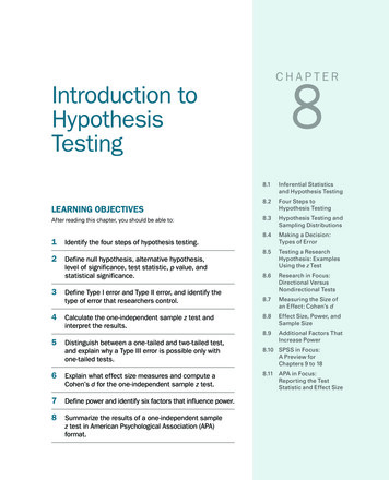
Standard Normal DistributionIThe following slide shows the table for the standard normaldistribution. On the vertical and horizontal axes you read the z-point(respectively the tenth and the hundredth), while inside the box youread the corresponding probabilityIThe blue box shows the point we used to compute the probability inthe previous slideIMake sure you can answer the following questions before going aheadIIIQuestion 1: what is the probability that the standard normal will give arealization below 1?Question 2: what is the point z below which the standard normal has0,95 probability to occur?Question 3: what is the probability that the standard normal will give arealization above (not below) -0.5Michele Piffer (LSE)Hypothesis Testing for BeginnersAugust, 201122 / 53
Michele Piffer (LSE)Hypothesis Testing for BeginnersAugust, 201123 / 53
Standard Normal DistributionIAnswers to our previous questionsIIII1) Prob(Z 1) 0, 84132) z so that Prob(Z z) 0, 95 is 1, 643) 1 Prob(Z 0.5) 0, 6915Last, make sure you understand the following theorem: if X isnormally distributed with expected value µ and varianceσ 2 , then if 2you subtract µ from X and divide everything by σ σ you obtaina new variable, which is a standard normal:Given X N(µ, σ 2 ) Michele Piffer (LSE)X µ N(0, 1) ZσHypothesis Testing for BeginnersAugust, 201124 / 53
Normal DistributionIWe are finally able to answer our question from a few slides before:what is the value of Prob(X 7) and Prob(8 X 10) givenX N(8, 16)?IDo we have a table for this special normal variable with E(x) 8 andVar(x) 16? No! But we don’t need it: we can do a transformation toX and exploit the table of the standard normalIRemembering that you can add/subtract or multiply/divide both sidesof an inequality, we obtain.Michele Piffer (LSE)Hypothesis Testing for BeginnersAugust, 201125 / 53
Normal DistributionProb(X 7) Prob(X 8 7 8) Prob(X 8 1) 1X 8X 8 ) Prob( 0, 25) Prob(444IThe theorem tells us that the variable X σ µ X 4 8 is a standardnormal, which greatly simplifies our question to: what is theprobability that a standard normal has a realization on the left ofpoint 0, 25 ? We know how to answer this question. From the tablewe getProb(X 7) Prob(Z 0, 25) 1 Prob(Z 0.25) 1 0, 5987 0.4013 40, 13%Michele Piffer (LSE)Hypothesis Testing for BeginnersAugust, 201126 / 53
Normal DistributionILet’s now compute the other probability:Prob(8 X 10) Prob(X 10) Prob(X 8) 8 810 8) Prob(Z ) Prob(Z 44 Prob(Z 0.5) Prob(Z 0) 0, 6915 0.5 0, 1915 19, 15%ITo sum up, a normal distribution with expected value 8 and variance16 could have realizations from to . But we now know thatthe probability that X will be lower than 7 is 40,13 %, while theprobability that it will be in the interval [8,10] is 19,15 %Michele Piffer (LSE)Hypothesis Testing for BeginnersAugust, 201127 / 53
Normal DistributionIGraphically, given X N(8, 16)IExercise: show that Prob(X 11) 22, 66%Michele Piffer (LSE)Hypothesis Testing for BeginnersAugust, 201128 / 53
Hypothesis TestingIWe are finally able to use what we have seen so far to do hypothesistesting. What is this about?IIn all the exercises above, we assumed to know the parameter valuesand investigated the properties of the distribution (i.e. we knew thatµ 8 and σ 2 16). Of course, knowing the true values of theparameters is not a straightforward taskIBy inference we mean research of the values of the parameters givensome realizations of the variable (i.e. given some data)Michele Piffer (LSE)Hypothesis Testing for BeginnersAugust, 201129 / 53
Hypothesis TestingIThere are two ways to proceed. The first one is to use the data toestimate the parameters, the second is to guess a value for theparameters and ask the data whether this value is true. The formerapproach is estimation, the latter is hypothesis testingIIn the rest of the notes we will do hypothesis testing on the expectedvalue of a normal distribution, assuming that the true variance isknown. There are of course tests on the variance, as well as all kindsof testsMichele Piffer (LSE)Hypothesis Testing for BeginnersAugust, 201130 / 53
Hypothesis TestingIConsider the following scenario. We have a normal random variablewith expected value µ unknown and variance equal to 16IWe are told that the true value for µ is either 8 or 25. For someexternal reason we are inclined to think that µ 8, but of course wedon’t really know for sure.IWhat we have is one realization of the random variable. The point is,what is this information telling us? Of course, the closer is therealization to 8 and the more I would be willing to conclude that thetrue value is 8. Similarly, the closer the realization is to 25 and themore I would reject that the hypothesis that µ 8Michele Piffer (LSE)Hypothesis Testing for BeginnersAugust, 201131 / 53
Hypothesis TestingIHow do we use the data to derive some meaningful procedure forinferring whether my data is supporting my null hypothesis of µ 8or is rejecting it in favor of the alternative µ 25?ILet’s first put things formally:X N(µ, 16) , with H0 : µ 8 vs. Ha : µ 25ICall x 0 the realization of X which we have and which we use to doinference. What is the distribution that has generated this point,X N(8, 16) or X N(25, 16)?Michele Piffer (LSE)Hypothesis Testing for BeginnersAugust, 201132 / 53
Hypothesis TestingIIf null hypothesis is true, the realization x 0 comes fromIIf alternative hypothesis is true, the realization x 0 comes fromMichele Piffer (LSE)Hypothesis Testing for BeginnersAugust, 201133 / 53
Hypothesis TestingIThe key intuition is: how far away from 8 must the realization be forus to reject the null hypothesis that the true value of µ is 8?ISuppose x 0 12. In this case x 0 is much more likely to come fromX N(8, 16) rather than from X N(25, 16). Similarly, if x 0 55then this value is much more likely to come from X N(25, 16)rather than from X N(8, 16)IThe procedure is to choose a point c (called critical value) and thenreject H0 if x 0 c, while not reject H0 if x 0 c. The point is to findthis c in a meaningful wayMichele Piffer (LSE)Hypothesis Testing for BeginnersAugust, 201134 / 53
Hypothesis TestingIStart with the following exercise. For a given c, what is theprobability that we reject H0 by mistake, i.e., when the true value forµ was actually 8? As we have seen, this is nothing but thee areaunder X N(8, 16) on the interval [c, ]Michele Piffer (LSE)Hypothesis Testing for BeginnersAugust, 201135 / 53
Hypothesis TestingIGiven c, we also know how to compute this probability. Under H0 , itis simply Prob(X c) Prob(Z c 84 )IWhat we just did is: given c, compute the probability of rejecting H0by mistake. The problem is that we don’t have c yet, that’s what weneed to compute!IA sensible way to choosing c is to do the other way around: find c sothat the probability of rejecting H0 by mistake is a given number,which we choose at the beginning. In other words, you choose withwhich probability of rejecting H0 by mistake you want to work andthen you compute the corresponding critical valueMichele Piffer (LSE)Hypothesis Testing for BeginnersAugust, 201136 / 53
Hypothesis TestingIIn jargon, the probability of rejecting H0 by mistake is called “type 1error”, or level of significance. It is expressed with the letter αIOur problem of finding a meaningful critical value c has been solved:at first, choose a confidence interval. Then find the point ccorresponding to the interval α. Having c, one only needs to compareit to the realization x 0 from the data. If x 0 c, then we reject H0 8,knowing that we might be wrong in doing so with probability αIThe most frequent values used for α are 0.01, 0,05 and 0,1Michele Piffer (LSE)Hypothesis Testing for BeginnersAugust, 201137 / 53
Hypothesis TestingILet’s do this with our example. Suppose we want to work with a levelof significance of 1 %IThe first thing to do is to find the critical vale c which, if H0 wastrue, would have 1 % probability on the right. Formally, find c so that0, 01 Prob(X c) Prob(Z Ic 8)4What is the point of the standard normal distribution which has areaof 0,01 on the right? This is the first value we saw when weintroduced the N(0,1) distribution. The value was 2,33:0, 01 Prob(Z Imposec 84Michele Piffer (LSE)c 8) Prob(Z 2, 33)4 2, 33 and obtain c 17, 32.Hypothesis Testing for BeginnersAugust, 201138 / 53
Hypothesis TestingIAt this point we have all we need to run our test. Suppose that therealization from X that we get is 15. Is x 0 15 far enough from µ 8to lead us to reject H0 ? Clearly 15 17, 32 , which means that wecannot reject the hypothesis that µ 8ISuppose we run the test with another realization of X, say x 0 20. Is20 sufficiently close to µ 25 to lead us to reject H0 ? Of course it is,given that 20 is above the critical c 17, 32Michele Piffer (LSE)Hypothesis Testing for BeginnersAugust, 201139 / 53
Hypothesis TestingINote that when rejecting H0 we cannot be sure at 100% that the truevalue for the parameter µ is not 8. Similarly, when we fail to reject H0we cannot be sure at 100 % that the true value for µ is actually 8.IWhat we know is only that, in doing the test several times, we wouldmistakenly reject µ 8 with α 0.01 probability.Michele Piffer (LSE)Hypothesis Testing for BeginnersAugust, 201140 / 53
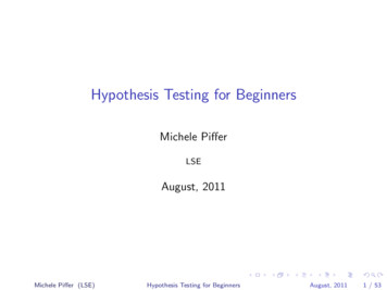
Hypothesis TestingIOur critical value c would have been different, had we chosen to workwith a different level of significance. For instance, the critical valuefor α 0, 05 is 14,56, while the critical value for α 0, 1 is 13,12(make sure you know how to compute these values)α0.010.050.10Ic17.3214.5613.12Suppose that the realization of X is 15. Do we reject H0 whenworking with a level of significance of 1 %? No. But do we reject it ifwe work with a level of significance of 10 %? Yes! The higher theprobability that we accept in rejecting H0 by mistake and the morelikely it is that we reject H0Michele Piffer (LSE)Hypothesis Testing for BeginnersAugust, 201141 / 53
Hypothesis TestingMichele Piffer (LSE)Hypothesis Testing for BeginnersAugust, 201142 / 53
Hypothesis TestingIIf, given x 0 , the outcome of the test depends on the level ofsignificance chosen, can we find a probability p so that we will rejectH0 for all levels of significance from 100 % down to p?ITo see why this question is interesting, compute the probability p onthe right of x 0 15. We will be able to reject H0 for all critical valueslower than x 0 , or equivalently, for all levels of significance higher thanp15 8) Prob(Z 1, 75) 4 1 Prob(Z 1, 75) 0, 0401p Prob(X x 0 ) Prob(Z Michele Piffer (LSE)Hypothesis Testing for BeginnersAugust, 201143 / 53
Hypothesis TestingMichele Piffer (LSE)Hypothesis Testing for BeginnersAugust, 201144 / 53
Hypothesis TestingIIf we have chosen α p, then it means that x 0 c and we cannotreject H0IIf we have chosen an α p, then it means that x 0 c and we canreject H0IIn our example, we can reject H0 for all levels of significanceα 4, 01%IThe probability p is called p-value. The p-value is the lowest level ofsignificance which allows to reject H0 . The lower p and the easier willbe to reject H0 , since we will be able to reject H0 with lowerprobabilities of rejecting it by mistake. In other words, the lower pand the more confident you are in rejecting H0Michele Piffer (LSE)Hypothesis Testing for BeginnersAugust, 201145 / 53
Hypothesis TestingIOur last step involves the following question. What if the true valuefor µ was actually 25? What is the probability that we mistakenly failto reject H0 when the true µ was actually 25?IGiven what we saw so far this should be easy: it is the area on theregion [ , c] under the pdf of the alternative hypothesis:Michele Piffer (LSE)Hypothesis Testing for BeginnersAugust, 201146 / 53
Hypothesis TestingIIn jargon, the probability of not rejecting H0 when it is actually wrongis called “type 2 error”. It is expressed by the letter βILet’s go back to our example. At this point you should be able tocompute β easily. Under Ha we haveβ Prob(X c) Prob(X 17, 32) X 2517, 32 25 Prob( ) Prob(Z 1, 92) 0, 027444ILast, what is the probability that we reject H0 when it was actuallywrong and the true one was Ha ? It is obviously the area underX N(25, 16) in the interval [c, ], or equivalently,1 β 0, 9726. This is the power of the testMichele Piffer (LSE)Hypothesis Testing for BeginnersAugust, 201147 / 53
Hypothesis TestingIThe power of a test is the probability that we correctly reject the nullhypothesis. It is expressed by the letter πMichele Piffer (LSE)Hypothesis Testing for BeginnersAugust, 201148 / 53
Hypothesis TestingITo sum up, the procedure for running an hypothesis testing requiresto:IIIIIIIChoose a level of significance αCompute the corresponding critical value and define the critical regionfor rejecting or not rejecting the null hypothesisObtain the realization of your random variable and compare it to cIf you reject H0 , then you know that the probability that you are wrongin doing so is αGiven H1 and the level c, compute the power of the testIf you reject the H0 in favor of H1 , then you know that you are right indoing so with probability given by πAlternatively, one can compute the p-value corresponding to therealization of X given by the data and infer all levels of significance upto which you can reject H0Michele Piffer (LSE)Hypothesis Testing for BeginnersAugust, 201149 / 53
Hypothesis TestingIIn the example seen so far, choosing α 0, 01, we reject H0 for allx 0 17, 32 and do not reject it for all x 0 17, 32Michele Piffer (LSE)Hypothesis Testing for BeginnersAugust, 201150 / 53
Hypothesis TestingITo conclude, three remarks are necessary:IRemark 1: What if we specify that the alternative hypothesis is not asingle point, but it is simply Ha : µ 6 8?ISuch a test is called two-sided test, compared to the one-sided testseen so far. Nothing much changes, other than the fact that therejection region will be divided into three parts. Find c1 .c2 so thatα Prob(X c1 or X c2 ) 1 Prob(c1 X c2 )IThen, you reject H0 if x 0 lies outside the interval [c1 , c2 ] and do notreject H0 otherwiseMichele Piffer (LSE)Hypothesis Testing for BeginnersAugust, 201151 / 53
Hypothesis TestingIRemark 2: why should one use only a single realization of X ? Doesn’tit make more sense to extract n observations and then compute theaverage?IYes, of course. Nothing much changes in the interpretation. The onlynote of caution is on the distribution used. It is possible to show that,if X N(µ, σ 2 ), thenσ2X N(µ, )n1 Pnwith X n i 1 XiIThe construction of the test follows the same steps, but you have touse the new distributionMichele Piffer (LSE)Hypothesis Testing for BeginnersAugust, 201152 / 53
Hypothesis TestingIRemark 3: so far we assumed that we knew the true value of σ 2 . Butwhat is it? Shouldn’t we estimate it? Doesn’t this change something?IYes, or course. One can show that the best thing to do is tosubstitute σ 2 with the following statistic:ns2 1 X(X1 X )2n 1i 1IThe important difference in this case is that the statistics will notfollow the normal distribution, but a different distribution (known asthe t distribution). The logical steps for constructing the test are thesame. For the details, have a look at a book of statisticsMichele Piffer (LSE)Hypothesis Testing for BeginnersAugust, 201153 / 53
\probability density functions". Nevertheless, the profession expects him to know the basics of hypothesis testing. These notes o er a very simpli ed explanation of the topic. The ambition is to get the ideas through the mind of someone whose knowledge of statistics is limited to the fact that a probability cannot be bigger than one.