Transcription
Guide to Spectrum andSignal Analysis
CONTENTSINTRODUCTION.4Frequency Domain / Time Domain.4SPECTRUM ANALYZERS.6Signal Analyzers.7Basic Operation.7Characteristics.8Frequency Range.8Frequency Resolution.9Sweep Speed.12Sensitivity and Noise Figure.12Video Filtering or Averaging.13Signal Display Range.14Dynamic Range.16Frequency Accuracy.16SIGNAL ANALYZERS.17APPLICATIONS.18Amplitude Modulation.18Modulation Frequency – fm.22Modulation Distortion.24Frequency Modulation.26Bandwidth of FM Signals.27FM Measurements with a Spectrum Analyzer.29AM Plus FM (Incidental FM).32PULSE AND PULSE MODULATED SIGNALS.33Pulse Response.34Pulse Spectrum.35MEASUREMENT EXAMPLES.35Intermodulation Distortion.35C/N measurement.36Occupied Frequency Bandwidth.37a) XdB Down method.37b) N% method.38Adjacent Channel Leakage Power.39Burst Average Power.402 Guide to Spectrum and Signal Analysis
APENDIX ASpectrum Analyzer Conversion Factors. 42SWR – Reflection Coefficient – Return Loss. 43Power Measurement. 44APPENDIX BAmplitude Modulation. 45APPENDIX CFrequency Modulation. 48Bessel Functions.APPENDIX DPulse Modulation. 51APPENDIX EIntermodulation Distortion / Intercept Points. 53While careful attention has been taken to ensure the contents of this booklet are accurate, Anritsu cannotaccept liability for any errors or omissions that occur. We reserve the right to alter specifications of productswithout prior notice.www.anritsu.com 3
INTRODUCTIONEngineers and technicians involved in modern RF or microwave communications have many measuringinstruments at their disposal, each designed for specific measurement tasks. Among those available are:a) T he Oscilloscope – primarily developed for measuring and analyzing signal amplitudes in the timedomain. (Voltage vs. time) Often 2, 4 or more channels of voltage vs. time can be viewed on the samedisplay to show the relationships between signals. Extensive methods to trigger signals are oftenavailable to capture and display rare events.b) T he Spectrum Analyzer – designed to measure the frequency and amplitude of electromagneticsignals in the frequency domain. (Frequency vs. time) Most modern analyzers also have the capabilityto demodulate analog modulated signals. Spectrum analyzers are the most versatile tools available tothe RF engineer. This guide will describe the critical performance characteristics of spectrum andsignal analyzers, the types of signals measured, and the measurements performedc) T he Signal Analyzer – invaluable for measuring the modulation characteristics of complex signals.These units capture and process blocks of spectrum to reveal amplitude and phase relationshipsbetween signals. Newer models provide demodulation of digitally modulated signals used in most oftoday’s communications systems.d) T he Signal Generator – an essential item of equipment for any communications test laboratory orworkshop. The cost of a signal generator largely depends on the additional functions and facilitiesavailable as well as the type and quality of the frequency reference used.e) T he Field Strength Meter (F.S.M.) – display the power density of an electrical signal incident on acalibrated antenna and thus give a direct reading of field strength in dBµV/m.f) T he Frequency Counter – a digitally based instrument that measures and displays the frequency ofincoming signals. Some models can also count ‘pulse’ and ‘burst’ signals.Frequency Domain / Time DomainAs mentioned in the introduction, electromagnetic signals can be displayed either in the time domain, byan oscilloscope, or in the frequency domain using a spectrum or signal analyzer. Traditionally, the timedomain is used to recover the relative timing and phase information required to characterize electricalcircuit behavior. Many circuit elements such as amplifiers, modulators, filters, mixers and oscillators arebetter characterized by their frequency response information. This frequency information is best obtainedby analysis in the frequency domain. Modern Oscilloscopes provide frequency domain display modesand modern Spectrum and Signal analyzers provide time domain displays. One key difference betweenoscilloscopes and spectrum/signal analyzers is the resolution of the vertical axis. Oscilloscopes providehigh resolution along the time axis but low (8 bit) amplitude resolution. Spectrum and signal analyzersprovide high (16 bit or more) amplitude resolution to see small signals in the presence of large signals.4 Guide to Spectrum and Signal Analysis
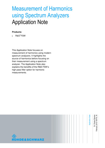
In order to visualize these ‘domains’ refer to Figure 1.aftxyFigure 1This represents an electromagnetic signal as a 3 dimensional model using:(i) a time axis (t)(ii) a frequency axis (f) and(iii) an amplitude axis (a)Observing from position X produces an amplitude time display where the resultant trace is the sum of theamplitudes of each signal present. This time domain view facilitates analysis of complex signals, butprovides no information on the individual signal components (Figure re 2www.anritsu.com 5
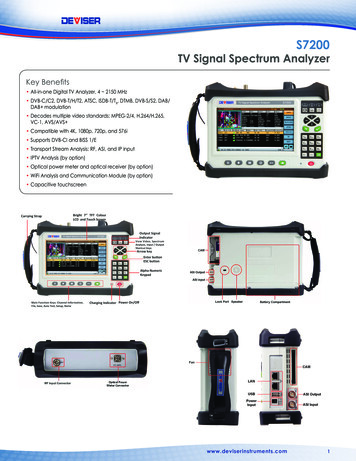
Viewing the model in Figure 1 from position Y, however, produces an amplitude vs. frequency displayshowing each component of the signal in the complex waveform. Observation in this frequency domainpermits a quantitative measurement of the frequency response, spurious components and distortion ofcircuit elements (Figure 3).Figure 3SPECTRUM ANALYZERSA Spectrum Analyzer is a swept tuned analyzer is tuned by electronically sweeping its input over thedesired frequency range thus, the frequency components of a signal are sampled sequentially in time(Figure 4). Using a swept tuned system enables periodic and random signals to be displayed but doesnot allow for transient responses.RF InputAttenuatorMixerIF GainIF FilterInputSignalLogAmpEnvelope VideoDetector FilterADCPre-selector, orLow-pass PUFigure 4Display6 Guide to Spectrum and Signal Analysis
Signal AnalyzersSignal analyzers sample a range of frequencies simultaneously, thus preserving the time dependencyand phase between signals. This technique allows both transient and periodic / random signals to bedisplayed (Figure 5). Signal Analyzers and Spectrum analyzers have very similar RF block diagrams,differing in frequency range (bandwidth) of the IF processing. The high bandwidth processing offersmany advantages, but at increased cost.RF InputAttenuatorMixerIF GainInputSignalADCDDCI/QPre-selector, orLow-pass FilterStepSynthesizerCPU / FFTReferenceOscillatorFigure 5DisplayBasic OperationBoth spectrum analyzers and signal analyzers are based on a super heterodyne receiver principle(Figure 6). The input signal, fIN, is converted to an intermediate frequency, fIF, via a mixer and a tunablelocal oscillator fLO. When the frequency difference between the input signal and the local oscillator isequal to the intermediate frequency then there is a response on the display.1st MixerB.P.F2nd Mixer3rd VertHorizFigure 6CPUDisplayfIN fLO fIFwww.anritsu.com 7
This is the basic tuning equation that determines the frequency range of a spectrum/signal analyzer.Using the super heterodyne technique enables high sensitivity through the use of intermediate frequency(IF) amplifiers and extended frequency range by using the harmonics of the local oscillator (LO). Thistechnique is not, however, real time and sweep rates must be consistent with the IF filter bandwidthcharge time.CharacteristicsSpectrum and signal analyzers have the following characteristics:a)b)c)d)e)f)g)h)i)Wide frequency range.Amplitude and frequency calibration via internal calibration source and error correction routines.Flat frequency response where amplitude is independent of frequency.Good frequency stability using synthesized local oscillators and reference source.Low internal distortion.Good frequency resolution.High amplitude sensitivity.Linear and logarithmic display modes for amplitude (voltage and dB scaling).Absolute and relative measurement capabilities.Frequency RangeThe lower frequency limit of a spectrum analyzer is determined by the sideband noise of the localoscillator. The local oscillator feedthrough occurs even when there is no input signal present.The sensitivity at the lower frequency is also limited by the LO. sideband noise. Figure 7 shows typicaldata of average noise level vs. frequency for two IF bandwidths.10 kHz RBW1 kHz RBWFigure 78 Guide to Spectrum and Signal Analysis
It should be noted however, that as the IF bandwidth is reduced so the time to sweep a given frequencyrange increases since the charge time of the IF filter increases. This means that the sweep time isincreased to allow the IF filter to respond and therefore present an undistorted signal to the detector. Thesevariables are generally taken into account automatically and are referred to as ‘coupling’. Beyond thedetector can be more filtering known as Video Bandwidth and this can also be coupled to IF bandwidthand sweep time. These functions are coupled together since they are all inter dependent on each other,i.e. change one parameter setting and it affects the others.An additional facility available on most modern analyzers is a Zero Frequency Span mode. As mentionedearlier, most analyzers are based on the super heterodyne receiver design, where the local oscillator isswept continuously. If the local oscillator is manually tuned, the spectrum analyzer becomes a fixedtuned receiver whose frequency is determined by that of the local oscillator. In this mode the analyzerwill display the time domain function since the frequency component is fixed even though the scangenerator is still sweeping the display i.e. the display is now amplitude vs. time (Figure 8).Figure 8Frequency ResolutionThe frequency resolution (typically called “resolution bandwidth”) of a spectrum/signal analyzer is its abilityto separate and measure two signals in close proximity. This frequency resolution is determined by threeprimary factors:a) the IF filter bandwidth usedb) the shape of the IF filter andc) the sideband noise of the IF filterwww.anritsu.com 9
The IF bandwidth is normally specified by Δf at 3 dB (Figure 9). From this it can be seen that the narrowerthe filter bandwidth the greater the frequency resolution. However, as mentioned earlier, as the IF bandwidth is reduced so the charge time for the filter increases hence increasing the sweep time. As an example, narrow IF bandwidths are required to distinguish the sidebands of amplitude and frequencymodulated signals (Figure 10).Δf @ –3 dBFigure 9Figure 1010 Guide to Spectrum and Signal Analysis
When measuring close in spurious components, the shape of the IF filter becomes important. The filterskirt inclination is determined by the ratio of the filter bandwidth at –60 dB to that at –3 dB (Figure 11).Δf @ –3 dBΔf @ –60 dBFigure 11This skirt inclination is known as the ‘shape factor’ of the filter and provides a convenient guide to the filterquality. The most common type of IF filter is known as the Gaussian filter, since its shape can be de rivedfrom the Gaussian function of distribution. Typical shape factor values for Gaussian filters are 12:1/ 60 dB:3dB, while some spectrum analyzers utilize digital filters where the shape factor can be as low as 3:1. Digitalfilters appear to be better in terms of frequency resolution, but they do have the drawback of sharplyincreasing the scan time required to sweep a given frequency range. Figure 12 shows the effects ofscanning too fast for a given IF bandwidth filter. As the scan time decreases, the displayed amplitudedecreases and the apparent bandwidth increases. Consequently, frequency resolution and amplitudeuncertainty get worse, and some analyzers will warn you that you are now in an ‘UNCAL’ mode.Figure 12www.anritsu.com 11
A spectrum analyzer’s ability to resolve two closely spaced signals of unequal amplitude is not onlydependent on the IF filter shape factor. Noise sidebands can reduce the resolution capabilities since theywill appear above the skirt of the filter and so reduce the out of band rejection of the filter.Sweep SpeedSpectrum analyzers, incorporating swept local oscillators have the issue of needing to manage the sweepspeed to prevent uncalibrated displays. Signal analyzers do not. Blocks of spectrum are processedtogether in a signal analyzer. See Figure 5. The sample rate of the A to D converter determines the spanof spectrum that can be processed. The span is approximately ½ the A to D sample rate. The difference insweep speed performance between the spectrum analyzer mode and signal analyzer mode is especiallyvisible when very narrow resolution bandwidths are used. Most modern analyzers combine swept spectrumand signal analyzer technology. The spectrum analyzer mode offers very wide span views and the signalanalyzer mode offers fast spectrum displays for narrow spans. The sweep speed for signal analyzerbased spectrum displays depends on the FFT computation speed. Dedicated FFT processing circuitrycan speed up spectrum display rates to support searching for intermittent signals.Sensitivity and Noise FigureThe sensitivity of a spectrum analyzer is defined as its ability to detect signals of low amplitude. Themaximum sensitivity of the analyzer is limited by the noise generated internally. This noise consists ofthermal (or Johnson) and non-thermal noise. Thermal noise power is expressed by the following equation:wherePN Noise power (in Watts)k Boltzman’s constant (1.38 x 10²³ JK–1)T Absolute temperature (Kelvin)B System Bandwidth (Hz)PN kTBFrom this equation it can be seen that the noise level is directly proportional to the system bandwidth.Therefore, by decreasing the bandwidth by an order of 10 dB the system noise floor is also decreased by10 dB (Figure 13).10 kHz RBW1 kHz RBWFigure 1312 Guide to Spectrum and Signal Analysis
When comparing spectrum analyzer specifications it is important that sensitivity is compared for equalbandwidths since noise varies with bandwidth.An alternative measure of sensitivity is the noise factor FN:FN (S/N)IN / (S/N)OUTwhere S Signal and N NoiseFNF (S/N)(S/N)IN /(F10 log) dBOUT of merit weN can derive the noise figure as:Since the noise factor is a dimensionless figureF 10 log (FN) dBUsing the equation PN kTB it is possible to calculate the theoretical value of absolute sensitivity for agiven bandwidth. For example, if a spectrum analyzer generates no noise products at a temperature of17 degrees Celsius, referred to a 1Hz bandwidth, then:absolute sensitivity 1.38 x 10–23 x 290 4x10²¹ W/Hz –174dBm/HzTo determine the noise figure of a typical spectrum analyzer where the average noise floor is specifiedas 120 dBm referred to a 300 Hz bandwidth:–120 dBm –174 dBm/Hz 10 log 300 F (dB)F (dB) –120 174 –24.8Noise Figure 29.2 dBVideo Filtering or AveragingVery low level signals can be difficult to distinguish from the average internal noise level of many spectrumanalyzers. Since analyzers display signal plus noise, some form of averaging or filtering is required toassist the visual detection process. As mentioned earlier, a video filter is a low pass, post detection filterthat averages the internal noise of the analyzer.Because spectrum analyzers measure signal plus noise, the minimum signal power that can be displayedis the same as the average noise power of the analyzer. From this statement it would appear that thesignal would be lost in the analyzer noise but:if signal power average noise powerthen by definition, the minimum signal power that can be displayed will be:WhereS signal powerN average noise powerS N 2Nwww.anritsu.com 13
When the signal power is added to the average noise power, the resultant signal power displayed will be3 dB greater (Figure 14). This 3 dB difference is sufficient for low level signal identification.Figure 14Signal Display RangeThe signal display range of a spectrum/signal analyzer with no input attenuation is dependent on two keyparameters.a) The minimum resolution bandwidth available and hence the average noise level of the analyzer andb) The maximum level delivered to the first mixer that does not introduce distortion or inflict permanentdamage to the mixer performance.Typical values for these two factors are shown in Figure 15.As the input level to the first mixer increases so the detected output from the mixer will increase. However,since the mixer is a semiconductor diode the conversion of input level to output level is constant untilsaturation occurs. At this point the mixer begins to gain compress the input signal, and conversion revertsfrom linear to near logarithmic. This gain compression is not considered serious until it reaches 1 dB.Input levels that result in less than 1 dB gain compression are called linear input levels (Figure 16).Above 1 dB gain compression, the conversion law no longer applies and the analyzer is considered to beoperating nonlinearly and the displayed signal amplitude is not an accurate measure of the input signal.14 Guide to Spectrum and Signal Analysis
Distortion products are produced in the analyzer whenever a signal is applied to the input. These distortionproducts are usually produced by the inherent nonlinearity of the mixer. By biasing the mixer at an optimumlevel internal distortion products can be kept to a minimum. Typically, modern spectrum analyzer mixersare specified as having an 80 dB spurious free measurement range for an input level of –30 dBm.Obviously the analyzer will be subjected to input signals greater than –30 dBm and to prevent exceedingthe 1 dB compression point, an attenuator is positioned between the analyzer input and the first mixer.The attenuator automatically adjusts the input signal to provide the –30 dBm optimum level. 30 dBm Damage LevelTotalMeasurementRange–10 dBm 1 dB Gain Compression–30 dBmMax Input for Specified DistortionOptimum Operating Range(80 dB, Spurious-Free–110 dBmNoise Level (10 kHz BW)–120 dBmNoise Level (1 kHz BW)–130 dBmNoise Level (100 Hz BW)–140 dBmNoise Level (10 Hz BW)Figure 151 dBP inP outFigure 16www.anritsu.com 15
Dynamic RangeThe dynamic range of a spectrum/signal analyzer is determined by four key factors.i. Average noise level.This is the noise generated within the spectrum analyzer RF section, and is distributed equally acrossthe entire frequency range.ii. Residual spurious components.The harmonics of various signals are mixed together in complex form and converted to the IF signalcomponents which are displayed as a response on the display. Consequently, the displayed responseis present regardless of whether or not a signal is present at the input.iii. Distortion due to higher order harmonics.When the input signal level is high, spurious images of the input signal harmonics are generated dueto the nonlinearity of the mixer conversion.iv. Distortion due to two signal 3rd order intermodulation products.When two adjacent signals at high power are input to a spectrum/signal analyzer, intermodulationoccurs in the mixer paths. Spurious signals, separated by the frequency difference of the input signalsare generated above and below the input signals.The level range over which measurements can be performed without interference from any of thesefactors is the dynamic range. This represents the analyzers performance and is not connected with thedis play (or measurement) range. The four parameters that determine dynamic range can normally befound in the analyzer specifications.For simplicity, some analyzer specifications state the dynamic range as “Y dB for an input level of X dBm”.The following example shows how these parameters are related to dynamic range:Amplitude Dynamic Range: 70 dB for a mixer input signal level of –30 dBm (Atten. 0 dB) In order toachieve this value of dynamic range the following conditions are required:a) the IF bandwidth must be narrow enough such that the average noise level is better than –100 dBm.b) the residual spurious components must be less than –100 dBm.c) for an input level of 30 dBm the higher harmonic distortion must be better than –70 dB (i.e. better than–100 dBm).Analyzer manufacturers often relate the above specifications at a particular frequency or over a range offrequencies.Frequency AccuracyThe key parameter relating to frequency accuracy is linked to the type of reference source built into thespectrum/signal analyzer. SynthesizedThe analyzer local oscillator is phase locked to a very stable reference source, often temperaturecontrolled to prevent unwanted frequency drifting. In this case, a precision crystal is often used and theoverall frequency accuracy and stability, both short term and long term depend on its quality. Portableanalyzers, intended for outdoor use, often have GPS receivers that can significantly improve thestability of the internal local oscillator. Non SynthesizedThe analyzer local oscillator operates as a stand-alone voltage controlled source16 Guide to Spectrum and Signal Analysis
Signal AnalyzersSignal analyzers incorporate a wide bandwidth digitizer in the IF to capture a time block of spectrum for analysis.Frequency, time and phase relationships of signals can be analyzed within the bandwidth and time limits of thecaptured spectrum. Digital modulation can be characterized in many ways not possible with a swept tunedspectrum analyzer. Figure 17 compares the block diagrams for a spectrum analyzer and signal analyzer.Figure 18 show example time blocks of spectrum with a variety of modulations. A signal analyzer is oftenused to measure the characteristics of analog and digital modulation.RF InputAttenuatorMixerIF GainIF FilterLogAmpEnvelope VideoDetector FilterInputSignalADCSpectrumAnalyzerPre-selector, orLow-pass PURF CI/QDisplayPre-selector, orLow-pass FilterSynthesizerCPU / FFTReferenceOscillatorFigure 1710Display1Digital Data0Digital BasebandModulation SignalAmplitudetFrequencytPhasetBoth Amplitudeand PhasetU(t) U(t) sin(2πfct φ(t))AMFMPMFigure 18www.anritsu.com 17
Figure 19 shows a signal analyzer display of QPSK modulation in polar display format. The polar displayis called a constellation or vector diagram.QTb1 0 0 1 1 0 1 0 0 1InformationBits: 00 0 10 100111t–AAI-Data:0ItAQ-Data:0t–AT 2Tb0010QPSKFigure 19APPLICATIONSAs stated in the introduction, spectrum analyzers are used to display the frequency and amplitude ofsignals in the frequency domain. Efficient transmission of information is accomplished by a techniqueknown as modulation. This technique transforms the information signal, usually of low frequency, to ahigher carrier frequency by using a third, modulation signal. But why modulate the original signal? Thetwo primary reasons are:1) modulation techniques allow the simultaneous transmission of two or more low frequency, or baseband signals onto a higher, carrier frequency and2) high frequency antenna are small in physical size and more electrically efficient.In this section we will consider three common modulation formats: Amplitude Modulation or AM. Frequency Modulation or FM. Pulse Modulation or PM.Each modulation technique places emphasis on a particular area of the analyzer’s specification.Amplitude ModulationAs the name suggests, amplitude modulation is where the carrier signal amplitude is varied by anamount proportional to the amplitude of the signal wave and at the frequency of the modulation signal.The amplitude variation about the carrier is termed the modulation factor ‘m’. This is usually expressedas a percentage called the percent modulation, %M.The complex expression for an AM carrier shows that there are three signal elements.a) the unmodulated carrier.b) the upper sideband whose frequency is the sum of the carrier and the modulation frequency.c) the lower sideband whose frequency is the difference between the carrier and the modulationfrequency.18 Guide to Spectrum and Signal Analysis
The spectrum analyzer display enables accurate measurement of three key AM parameters. Modulation Factor m. Modulation Frequency fm. Modulation DistortionFigure 20 shows the time domain display of a typical AM signal. From this the modulation factor, m, canbe expressed as follows:mmm–EE–EcEmaxmaxE max –E cccmax E cEEcccEquation 1Since the modulation is symmetrical:–EEc E c –E minEmax–Emaxc E–EminEEccc –Emaxcmin–Emaxc min EEminEmaxmax EEminEminc E maxmaxminE2 Eccc 22Emax –E–EminEmaxm max –E minminEmaxminmm Emax E minE Eminmax E minminEmaxmaxEmaxEcEminEquation 2Equation 3Equation 4Figure 20Equation 4 is true for sinusoidal modulation. If we view the AM signal on a spectrum analyzer in linear(voltage) mode we obtain Figure 21.ES LSBES USBFigure 21From this the percentage modulation, %M, can be calculated as follows:%M (ES LSB ES USB)x 100EcEquation 5where Es Amplitude of the sideband (volts)Ec Amplitude of the carrier
displayed (Figure 5). Signal Analyzers and Spectrum analyzers have very similar RF block diagrams, differing in frequency range (bandwidth) of the IF processing. The high bandwidth processing offers many advantages, but at increased cost. Basic Operation Both spectrum analyzers and signal analyzers are based on a super heterodyne receiver principle