Transcription
Time Series: Autoregressive modelsAR, MA, ARMA, ARIMAMingda ZhangUniversity of Pittsburghmzhang@cs.pitt.eduOctober 23, 20181 / 77
Overview1 Introduction of Time SeriesCategories and TerminologiesWhite Noise and Random WalkTime Series Analysis2 ARIMA ModelsAR ProcessMA ProcessARMA ModelsARIMA Models3 ARIMA Modeling: A Toy Problem2 / 77
Time Series A time series is a sequential set of data points, measuredtypically over successive times. Time series analysis comprises methods for analyzing timeseries data in order to extract meaningful statistics and othercharacteristics of the data.3 / 77
Categories and Terminologies Time-domain vs. Frequency-domain– Time-domain approach: how does what happened today affectwhat will happen tomorrow?These approaches view the investigation of lagged relationshipsas most important, e.g. autocorrelation analysis.– Frequency-domain approach: what is the economic cyclethrough periods of expansion and recession?These approaches view the investigation of cycles as mostimportant, e.g. spectral analysis and wavelet analysis. This lecture will focus on time-domain approaches.4 / 77
Categories and Terminologies (cont.) univariate vs. multivariateA time series containing records of a single variable is termedas univariate, but if records of more than one variable areconsidered then it is termed as multivariate. linear vs. non-linearA time series model is said to be linear or non-lineardepending on whether the current value of the series is alinear or non-linear function of past observations. discrete vs. continuousIn a continuous time series observations are measured at everyinstance of time, whereas a discrete time series containsobservations measured at discrete points in time. This lecture will focus on univariate, linear, discrete timeseries.5 / 77
Components of a Time Series In general, a time series is affected by four components, i.e.trend, seasonal,cyclical and irregular components.90807060cents per pound110– TrendThe general tendency of a time series to increase, decrease orstagnate over a long period of time.200520102015The price of chicken: monthly whole bird spot price, Georgia docks, USTimecents per pound, August 2001 to July 2016, with fitted linear trend line.6 / 77
Components of a Time Series (cont.) In general, a time series is affected by four components, i.e.trend, seasonal,cyclical and irregular components.151050Quarterly Earnings per Share– Seasonal variationThis component explains fluctuations within a year during theseason, usually caused by climate and weather conditions,customs, traditional habits, etc.19601965197019751980Johnson & Johnson quarterly earnings per share,84 quarters, 1960-I to 1980-IV.Time7 / 77
Components of a Time Series (cont.) In general, a time series is affected by four components, i.e.trend, seasonal,cyclical and irregular components.7090110130– Cyclical variationThis component describes the medium-term changes caused bycircumstances, which repeat in cycles. The duration of a cycleCardiovascular Mortalityextends over longer periodof time.197019721974197619781980Average weekly cardiovascular mortality in Los Angeles County. There are508 six-day smoothed averages obtained by filtering daily values over the10 year period 1970-1979.8 / 77
Components of a Time Series (cont.) In general, a time series is affected by four components, i.e.trend, seasonal,cyclical and irregular components.– Irregular variationIrregular or random variations in a time series are caused byunpredictable influences, which are not regular and also do notrepeat in a particular pattern.These variations are caused by incidences such as war, strike,earthquake, flood, revolution, etc.There is no defined statistical technique for measuring randomfluctuations in a time series.9 / 77
Combination of Four Components Considering the effects of these four components, twodifferent types of models are generally used for a time series.– Additive ModelY (t) T (t) S(t) C (t) I (t)Assumption: These four components are independent of eachother.– Multiplicative ModelY (t) T (t) S(t) C (t) I (t)Assumption: These four components of a time series are notnecessarily independent and they can affect one another.10 / 77
Time Series Example: White Noise White Noise– A simple time series could be a collection of uncorrelatedrandom variables, {wt }, with zero mean µ 0 and finitevariance σw2 , denoted as wt wn(0, σw2 ). Gaussian White Noise– A particular useful white noise is Gaussian white noise, whereinthe wt are independent normal random variables (with mean 0and variance σw2 ), denoted as wt iid N (0, σw2 ). White noise time series is of great interest because if thestochastic behavior of all time series could be explained interms of the white noise model, then classical statisticalmethods would suffice.11 / 77
Time Series Example: Random Walk A random walk is the process by which randomly-movingobjects wander away from where they started. Consider a simple 1-D process:– The value of the time series at time t is the value of the seriesat time t 1 plus a completely random movement determinedby wt . More generally, a constant drift factor δ is introduced.Xt δ Xt 1 wt δt tXwii 1 20 020 40 60 80random walk010020030040050012 / 77
Time Series Analysis The procedure of using known data values to fit a time serieswith suitable model and estimating the correspondingparameters. It comprises methods that attempt to understandthe nature of the time series and is often useful for futureforecasting and simulation. There are several ways to build time series forecasting models,but this lecture will focus on stochastic process.– We assume a time series can be defined as a collection ofrandom variables indexed according to the order they areobtained in time, X1 , X2 , X3 , . . . t will typically be discrete andvary over the integers t 0, 1, 2, . . .– Note that the collection of random variables {Xt } is referred toas a stochastic process, while the observed values are referredto as a realization of the stochastic process.13 / 77
Measures of Dependence A complete description of a time series, observed as acollection of n random variables at arbitrary time pointst1 , t2 , . . . , tn , for any positive integer n, is provided by thejoint distribution function, evaluated as the probability thatthe values of the series are jointly less than the n constants,c1 , c2 , . . . , cn ; i.e.,Ft1 ,t2 ,.,tn (c1 , c2 , . . . , cn ) Pr (Xt1 c1 , Xt2 c2 , . . . , Xtn cn ). Unfortunately, these multidimensional distribution functionscannot usually be written easily. Therefore some informative descriptive measures can beuseful, such as mean function and more.14 / 77
Measurement Functions Mean function– The mean function is defined asZ µt µXt E [Xt ] xft (x)dx, provided it exists, where E denotes the usual expected valueoperator. Clearly for white noise series, µwt E [wt ] 0 for all t. For random walk with drift (δ 6 0),µXt E [Xt ] δt tXE [wi ] δti 115 / 77
Autocovariance for Time Series Lack of independence between adjacent values in time seriesXs and Xt can be numerically assessed. Autocovariance Function– Assuming the variance of Xt is finite, the autocovariancefunction is defined as the second moment productγ(s, t) γX (s, t) cov (Xs , Xt ) E [(Xs µs )(Xt µt )],for all s and t.– Note that γ(s, t) γ(t, s) for all time points s and t. The autocovariance measures the linear dependence betweentwo points on the same series observed at different times.– Very smooth series exhibit autocovariance functions that staylarge even when the t and s are far apart, whereas choppyseries tend to have autocovariance functions that are nearlyzero for large separations.16 / 77
Autocorrelation for Time Series Autocorrelation Function (ACF)– The autocorrelation function is defined asρ(s, t) pγ(s, t)γ(s, s)γ(t, t)– According to Cauchy-Schwarz inequality γ(s, t) 2 γ(s, s)γ(t, t),it’s easy to show that 1 ρ(s, t) 1. ACF measures the linear predictability of Xt using only Xs .– If we can predict Xt perfectly from Xs through a linearrelationship, then ACF will be either 1 or 1.17 / 77
Stationarity of Stochastic Process Forecasting is difficult as time series is non-deterministic innature, i.e. we cannot predict with certainty what will occurin the future. But the problem could be a little bit easier if the time series isstationary: you simply predict its statistical properties will bethe same in the future as they have been in the past!– A stationary time series is one whose statistical properties suchas mean, variance, autocorrelation, etc. are all constant overtime. Most statistical forecasting methods are based on theassumption that the time series can be renderedapproximately stationary after mathematical transformations.18 / 77
Which of these are stationary?19 / 77
Strict Stationarity There are two types of stationarity, i.e. strictly stationary andweakly stationary. Strict Stationarity– The time series {Xt , t Z} is said to be strictly stationary ifthe joint distribution of (Xt1 , Xt2 , . . . , Xtk ) is the same as thatof (Xt1 h , Xt2 h , . . . , Xtk h ).– In other words, strict stationarity means that the jointdistribution only depends on the “difference” h, not the time(t1 , t2 , . . . , tk ). However in most applications this stationary condition is toostrong.20 / 77
Weak Stationarity Weak Stationarity– The time series {Xt , t Z} is said to be weakly stationary if1 E [Xt2 ] , t Z;2 E [Xt ] µ, t Z;3 γX (s, t) γX (s h, t h), s, t, h Z.– In other words, a weakly stationary time series {Xt } must havethree features: finite variation, constant first moment, andthat the second moment γX (s, t) only depends on t s andnot depends on s or t. Usually the term stationary means weakly stationary, andwhen people want to emphasize a process is stationary in thestrict sense, they will use strictly stationary.21 / 77
Remarks on Stationarity Strict stationarity does not assume finite variance thus strictlystationary does NOT necessarily imply weakly stationary.– Processes like i.i.d Cauchy is strictly stationary but not weaklystationary. A nonlinear function of a strictly stationary time series is stillstrictly stationary, but this is not true for weakly stationary. Weak stationarity usually does not imply strict stationarity ashigher moments of the process may depend on time t. If time series {Xt } is Gaussian (i.e. the distribution functionsof {Xt } are all multivariate Gaussian), then weakly stationaryalso implies strictly stationary. This is because a multivariateGaussian distribution is fully characterized by its first twomoments.22 / 77
Autocorrelation for Stationary Time Series Recall that the autocovariance γX (s, t) of stationary timeseries depends on s and t only through s t , thus we canrewrite notation s t h, where h represents the time shift.γX (t h, t) cov (Xt h , Xt ) cov (Xh , X0 ) γ(h, 0) γ(h) Autocovariance Function of Stationary Time Seriesγ(h) cov (Xt h , Xt ) E [(Xt h µ)(Xt µ)] Autocorrelation Function of Stationary Time Seriesρ(h) pγ(t h, t)γ(t h, t h)γ(t, t) γ(h)γ(0)23 / 77
Partial Autocorrelation Another important measure is called partial autocorrelation,which is the correlation between Xs and Xt with the lineareffect of “everything in the middle” removed. Partial Autocorrelation Function (PACF)– For a stationary process Xt , the PACF (denoted as φhh ), forh 1, 2, . . . is defined asφ11 corr(Xt 1 , Xt ) ρ1φhh corr(Xt h X̂t h , Xt X̂t ),h 2where X̂t h and X̂t is defined as:X̂t h β1 Xt h 1 β2 Xt h 2 · · · βh 1 Xt 1X̂t β1 Xt 1 β2 Xt 2 · · · βh 1 Xt h 1– If Xt is Gaussian, then φhh is actually conditional correlationφhh corr(Xt , Xt h Xt 1 , Xt 2 , . . . , Xt h 1 )24 / 77
ARIMA Models ARIMA is an acronym that stands for Auto-RegressiveIntegrated Moving Average. Specifically,– AR Autoregression. A model that uses the dependentrelationship between an observation and some number oflagged observations.– I Integrated. The use of differencing of raw observations inorder to make the time series stationary.– MA Moving Average. A model that uses the dependencybetween an observation and a residual error from a movingaverage model applied to lagged observations. Each of these components are explicitly specified in the modelas a parameter. Note that AR and MA are two widely used linear models thatwork on stationary time series, and I is a preprocessingprocedure to “stationarize” time series if needed.25 / 77
Notations A standard notation is used of ARIMA(p, d, q) where theparameters are substituted with integer values to quicklyindicate the specific ARIMA model being used.– p The number of lag observations included in the model, alsocalled the lag order.– d The number of times that the raw observations aredifferenced, also called the degree of differencing.– q The size of the moving average window, also called the orderof moving average. A value of 0 can be used for a parameter, which indicates tonot use that element of the model. In other words, ARIMA model can be configured to performthe function of an ARMA model, and even a simple AR, I, orMA model.26 / 77
Autoregressive Models Intuition– Autoregressive models are based on the idea that current valueof the series, Xt , can be explained as a linear combination of ppast values, Xt 1 , Xt 2 , . . . , Xt p , together with a randomerror in the same series. Definition– An autoregressive model of order p, abbreviated AR(p), is ofthe formXt φ1 Xt 1 φ2 Xt 2 · · · φp Xt p wt pXφi Xt i wti 1where Xt is stationary, wt wn(0, σw2 ), and φ1 , φ2 , . . . , φp(φp 6 0) are model parameters. The hyperparameter prepresents the length of the “direct look back” in the series.27 / 77
Backshift Operator Before we dive deeper into the AR process, we need some newnotations to simplify the representations. Backshift Operator– The backshift operator is defined asBXt Xt 1 .It can be extended, B 2 Xt B(BXt ) B(Xt 1 ) Xt 2 , andso on. Thus,B k Xt Xt k We can also define an inverse operator (forward-shiftoperator ) by enforcing B 1 B 1, such thatXt B 1 BXt B 1 Xt 1 .28 / 77
Autoregressive Operator of AR Process Recall the definition for AR(p) process:Xt φ1 Xt 1 φ2 Xt 2 · · · φp Xt p wtBy using the backshift operator we can rewrite it as:Xt φ1 Xt 1 φ2 Xt 2 · · · φp Xt p wt(1 φ1 B φ2 B 2 · · · φp B p )Xt wt The autoregressive operator is defined as:φ(B) 1 φ1 B φ2 B 2 · · · φp B p 1 pXφj B j ,j 1then the AR(p) can be rewritten more concisely as:φ(B)Xt wt29 / 77
AR Example: AR(0) and AR(1) The simplest AR process is AR(0), which has no dependencebetween the terms. In fact, AR(0) is essentially white noise. AR(1) can be given by Xt φ1 Xt 1 wt .– Only the previous term in the process and the noise termcontribute to the output.– If φ1 is close to 0, then the process still looks like white noise.– If φ1 0, Xt tends to oscillate between positive and negativevalues.– If φ1 1 then the process is equivalent to random walk, whichis not stationary as the variance is dependent on t (andinfinite).30 / 77
AR Examples: AR(1) Process Simulated AR(1) Process Xt 0.9Xt 1 wt : MeanE [Xt ] 0 VarianceVar(Xt ) σw2(1 φ21 )31 / 77
AR Examples: AR(1) Process Autocorrelation Function (ACF)ρh φh132 / 77
AR Examples: AR(1) Process Partial Autocorrelation Function (PACF)φ11 ρ1 φ1φhh 0, h 233 / 77
AR Examples: AR(1) Process Simulated AR(1) Process Xt 0.9Xt 1 wt : MeanE [Xt ] 0 VarianceVar(Xt ) σw2(1 φ21 )34 / 77
AR Examples: AR(1) Process Autocorrelation Function (ACF)ρh φh135 / 77
AR Examples: AR(1) Process Partial Autocorrelation Function (PACF)φ11 ρ1 φ1φhh 0, h 236 / 77
Stationarity of AR(1) We can iteratively expand AR(1) representation as:Xt φ1 Xt 1 wt φ1 (φ1 Xt 2 wt 1 ) wt φ21 Xt 2 φ1 wt 1 wt. φk1 Xt k k 1Xφj1 wt jj 0 Note that if φ1 1 and supt Var(Xt ) , we have:Xt Xφj1 wt jj 0This representation is called the stationary solution.37 / 77
AR Problem: Explosive AR Process We’ve seen AR(1): Xt φ1 Xt 1 wt while φ1 1. What if φ1 1? Intuitively the time series will “explode”. However, technically it still can be stationary, because weexpand the representation differently and get:Xt Xφ j1 wt jj 1 But clearly this is not useful because we need the future(wt j ) to predict now (Xt ). We use the concept of causality to describe time series that isnot only stationary but also NOT future-dependent.38 / 77
General AR(p) Process An important property of AR(p) models in general is– When h p, theoretical partial autocorrelation function is 0:φhh corr(Xt h X̂t h , Xt X̂t ) corr(wt h , Xt X̂t ) 0.– When h p, φpp is not zero and φ11 , φ22 , . . . , φh 1,h 1 arenot necessarily zero. In fact, identification of an AR model is often best done withthe PACF.39 / 77
AR Models: Parameters Estimation Note that p is like a hyperparameter for the AR(p) process,thus fitting an AR(p) model presumes p is known and onlyfocusing on estimating coefficients, i.e. φ1 , φ2 , . . . , φp . There are many feasible approaches: Method of moments estimator (e.g. Yule-Walker estimator) Maximum Likelihood Estimation (MLE) estimator Ordinary Least Squares (OLS) estimator If the observed series is short or the process is far fromstationary, then substantial differences in the parameterestimations from various approaches are expected.40 / 77
Moving Average Models (MA) The name might be misleading, but moving average modelsshould not be confused with the moving average smoothing. Motivation– Recall that in AR models, current observation Xt is regressedusing the previous observations Xt 1 , Xt 2 , . . . , Xt p , plus anerror term wt at current time point.– One problem of AR model is the ignorance of correlated noisestructures (which is unobservable) in the time series.– In other words, the imperfectly predictable terms in currenttime, wt , and previous steps,wt 1 , wt 2 , . . . , wt q , are alsoinformative for predicting observations.41 / 77
Moving Average Models (MA) Definition– A moving average model of order q, or MA(q), is defined to beXt wt θ1 wt 1 θ2 wt 2 · · · θq wt q wt qXθj wt jj 1where wt wn(0, σw2 ), and θ1 , θ2 , . . . , θq (θq 6 0) areparameters.– Although it looks like a regression model, the difference is thatthe wt is not observable. Contrary to AR model, finite MA model is always stationary,because the observation is just a weighted moving averageover past forecast errors.42 / 77
Moving Average Operator Moving Average Operator– Equivalent to autoregressive operator, we define movingaverage operator as:θ(B) 1 θ1 B θ2 B 2 · · · θq B q ,where B stands for backshift operator, thus B(wt ) wt 1 . Therefore the moving average model can be rewritten as:Xt wt θ1 wt 1 θ2 wt 2 · · · θq wt qXt (1 θ1 B θ2 B 2 · · · θq B q )wtXt θ(B)wt43 / 77
MA Examples: MA(1) Process Simulated MA(1) Process Xt wt 0.8 wt 1 : Mean E [Xt ] 0 Variance Var(Xt ) σw2 (1 θ12 )44 / 77
MA Examples: MA(1) Process Autocorrelation Function (ACF)ρ1 θ11 θ12ρh 0, h 245 / 77
MA Examples: MA(1) Process Partial Autocorrelation Function (PACF)φhh ( θ1 )h (1 θ12 )2(h 1),h 11 θ146 / 77
MA Examples: MA(2) Process Simulated MA(2) Process Xt wt 0.5 wt 1 0.3 wt 2 : Mean E [Xt ] 0 Variance Var(Xt ) σw2 (1 θ12 θ22 )47 / 77
MA Examples: MA(2) Process Autocorrelation Function (ACF)ρ1 θ1 θ1 θ21 θ12 θ22ρ2 θ21 θ12 θ22ρh 0, h 348 / 77
General MA(q) Process An important property of MA(q) models in general is thatthere are nonzero autocorrelations for the first q lags, andρh 0 for all lags h q. In other words, ACF provides a considerable amount ofinformation about the order of the dependence q for MA(q)process. Identification of an MA model is often best done with theACF rather than the PACF.49 / 77
MA Problem: Non-unique MA Process Consider the following two MA(1) models:– Xt wt 0.2wt 1 ,wt iid N (0, 25),– Yt vt 5vt 1 ,vt iid N (0, 1)5.26 In fact, these two MA(1) processes are essentially the same.However, since we can only observe Xt (Yt ) but not noiseterms wt (vt ), we cannot distinguish them. Conventionally, we define the concept invertibility and alwayschoose the invertible representation from multiple alternatives. Note that both of them have Var(Xt ) 26 and ρ1 – Simply speaking, for MA(1) models the invertibility conditionis θ1 1.50 / 77
Comparisons between AR and MA Recall that we have seen for AR(1) process, if φ1 1 andsupt Var(Xt ) ,Xt Xφj1 wt jj 0 In fact, all causal AR(p) processes can be represented asMA( ); In other words, infinite moving average processesare finite autoregressive processes. All invertible MA(q) processes can be represented as AR( ).i.e. finite moving average processes are infiniteautoregressive processes.51 / 77
MA Models: Parameters Estimation A well-known fact is that parameter estimation for MA modelis more difficult than AR model.– One reason is that the lagged error terms are not observable. We can still use method of moments estimators for MAprocess, but we won’t get the optimal estimators withYule-Walker equations. In fact, since MA process is nonlinear in the parameters, weneed iterative non-linear fitting instead of linear least squares. From a practical point of view, modern scientific computingsoftware packages will handle most of the details after giventhe correct configurations.52 / 77
ARMA Models Autoregressive and moving average models can be combinedtogether to form ARMA models. Definition– A time series {xt ; t 0, 1, 2, . . . } is ARMA(p, q) if it isstationary andXt wt pXi 1φi Xt i qXθj wt j ,j 1where φp 6 0, θq 6 0, and σw2 0, wt wn(0, σw2 ).– With the help of AR operator and MA operator we definedbefore, the model can be rewritten more concisely as:φ(B)Xt θ(B)wt53 / 77
ARMA Problems: Redundant Parameters You may have observed that if we multiply a same factor onboth sides of the equation, it still holds.η(B)φ(B)Xt η(B)θ(B)wt For example, consider a white noise process Xt wt andη(B) (1 0.5B):(1 0.5B)Xt (1 0.5B)wtXt 0.5Xt 1 0.5wt 1 wt Now it looks exactly like a ARMA(1, 1) process! If we were unaware of parameter redundancy, we might claimthe data are correlated when in fact they are not.54 / 77
Choosing Model Specification Recall we have discussed that ACF and PACF can be used fordetermining ARIMA model hyperparamters p and q.AR(p)ACFTails offPACFCuts offafter lag pMA(q)Cuts offafter lag qARMA(p, q)Tails offTails offTails off Other criterions can be used for choosing q and q too, such asAIC (Akaike Information Criterion), AICc (corrected AIC) andBIC (Bayesian Information Criterion). Note that the selection for p and q is not unique.55 / 77
“Stationarize” Nonstationary Time Series One limitation of ARMA models is the stationarity condition. In many situations, time series can be thought of as beingcomposed of two components, a non-stationary trend seriesand a zero-mean stationary series, i.e. Xt µt Yt . Strategies– Detrending: Subtracting with an estimate for trend and dealwith residuals.Ŷt Xt µˆt– Differencing: Recall that random walk with drift is capable ofrepresenting trend, thus we can model trend as a stochasticcomponent as well.µt δ µt 1 wt Xt Xt Xt 1 δ wt (Yt Yt 1 ) δ wt Yt is defined as the first difference and it can be extended tohigher orders.56 / 77
Differencing One advantage of differencing over detrending for trendremoval is that no parameter estimation is required. In fact, differencing operation can be repeated.– The first difference eliminates a linear trend.– A second difference, i.e. the difference of first difference, caneliminate a quadratic trend. Recall the backshift operator Xt BXt 1 : Xt Xt Xt 1 Xt BXt (1 B)Xt 2 Xt ( Xt ) (Xt Xt 1 ) (Xt Xt 1 ) (Xt 1 Xt 2 ) Xt 2Xt 1 Xt 2 Xt 2BXt B 2 Xt (1 2B B 2 )Xt (1 B)2 Xt57 / 77
Detrending vs. Differencing90 80chicken110original 70 60 200520102015Timedetrended10 5 0resid(fit) 5 200520102015Timefirst difference3 1 0 1 2diff(chicken)2 2005 20102015Time58 / 77
From ARMA to ARIMA Order of Differencing– Differences of order d are defined as d (1 B)d ,where (1 B)d can be expanded algebraically for higherinteger values of d. Definition– A process Xt is said to be ARIMA(p, d, q) if d Xt (1 B)d Xtis ARMA(p, q).– In general, ARIMA(p, d, q) model can be written as:φ(B)(1 B)d Xt θ(B)wt.59 / 77
Box-Jenkins Methods As we have seen ARIMA models have numerous parametersand hyper parameters, Box and Jenkins suggests an iterativethree-stage approach to estimate an ARIMA model. ProceduresModel identification: Checking stationarity and seasonality,performing differencing if necessary, choosing modelspecification ARIMA(p, d, q).2 Parameter estimation: Computing coefficients that best fit theselected ARIMA model using maximum likelihood estimationor non-linear least-squares estimation.3 Model checking: Testing whether the obtained model conformsto the specifications of a stationary univariate process (i.e. theresiduals should be independent of each other and haveconstant mean and variance). If failed go back to step 1.1 Let’s go through a concrete example together for thisprocedure.60 / 77
Air Passenger DataMonthly totals of a US airline passengers, from 1949 to 196061 / 77
Model Identification As with any data analysis, we should construct a time plot ofthe data, and inspect the graph for any anomalies. The most important thing in this phase is to determine if thetime series is stationary and if there is any significantseasonality that needs to be handled. Test Stationarity– Recall the definition, if the mean or variance changes over timethen it’s non-stationary, thus an intuitive way is to plot rollingstatistics.– We can also make an autocorrelation plot, as non-stationarytime series often shows very slow decay.– A well-established statistical test called augmentedDickey-Fuller Test can help. The null hypothesis is the timeseries is non-stationary.62 / 77
Stationarity Test: Rolling StatisticsRolling statistics with sliding window of 12 months63 / 77
Stationarity Test: ACF PlotAutocorrelation with varying lags64 / 77
Stationarity Test: ADF Test Results of Augmented Dickey-Fuller TestItemTest Statisticp-value#Lags UsedNumber of Observations UsedCritical Value (1%)Critical Value (5%)Critical Value 1682-2.884042-2.578770 The test statistic is a negative number. The more negative it is, the stronger the rejection of the nullhypothesis.65 / 77
Stationarize Time Series As all previous methods show that the initial time series isnon-stationary, it’s necessary to perform transformations tomake it stationary for ARMA modeling.– Detrending– Differencing– Transformation: Applying arithmetic operations like log, squareroot, cube root, etc. to stationarize a time series.– Aggregation: Taking average over a longer time period, likeweekly/monthly.– Smoothing: Removing rolling average from original time series.– Decomposition: Modeling trend and seasonality explicitly andremoving them from the time series.66 / 77
Stationarized Time Series: ACF PlotFirst order differencing over logarithm of passengers67 / 77
Stationarized Time Series: ADF Test Results of Augmented Dickey-Fuller TestItemTest Statisticp-value#Lags UsedNumber of Observations UsedCritical Value (1%)Critical Value (5%)Critical Value 82501-2.884398-2.578960 From the ACF plot, we can see that the mean and stdvariations have much smaller variations with time. Also, the ADF test statistic is less than the 10% critical value,indicating the time series is stationary with 90% confidence.68 / 77
Choosing Model Specification Firstly we notice an obvious peak at h 12, because forsimplicity we didn’t model the cyclical effect. It seems p 2, q 2 is a reasonable choice. Let’s see threemodels, AR(2), MA(2) and ARMA(2, 2).69 / 77
AR(2): Predicted on Residuals RSS is a measure of the discrepancy between the data and theestimation model.– A small RSS indicates a tight fit of the model to the data.70 / 77
MA(2): Predicted on Residuals71 / 77
ARMA(2, 2): Predicted on Residuals Here we can see that the AR(2) and MA(2) models havealmost the same RSS but combined is significantly better.72 / 77
Forecasting The last step is to reverse the transformations we’ve done toget the prediction on original scale.73 / 77
SARIMA: Seasonal ARIMA Models One problem in the previous model is the lack of seasonality,which can be addressed in a generalized version of ARIMAmodel called seasonal ARIMA. Definition– A seasonal ARIMA model is formed by including additionalseasonal terms in the ARIMA models, de
Time Series A time series is a sequential set of data points, measured typically over successive times. Time series analysis comprises methods for analyzing time