Transcription
INVENTORY THEORYJAIME ZAPPONEAbstract. This paper is an introduction to the study of inventory theory.The paper illustrates deterministic and stochastic models. We present thederivation of each model, and we illustrate each model through the use ofexamples. We also learn about quantity discounts, and use the aforementionedmodels to understand a real world situation involving firecrackers. Finally,some of the economic practices of Zappone Manufacturing are analyzed. Itis shown how deterministic, stochastic and other simple models are not muchhelp to this company. Also included in this paper is a derivation of Leibniz’sRule, which helps in deriving the stochastic model. This paper assumes thereader to have a basic understanding of mathematical statistics.1. IntroductionKeeping an inventory (stock of goods) for future sale or use is common in business. In order to meet demand on time, companies must keep on hand a stockof goods that is awaiting sale. The purpose of inventory theory is to determinerules that management can use to minimize the costs associated with maintaininginventory and meeting customer demand. Inventory is studied in order to helpcompanies save large amounts of money. Inventory models answer the questions:(1) When should an order be placed for a product? (2) How large should eachorder be? The answers to these questions is collectively called an inventory policy. Companies save money by formulating mathematical models describing theinventory system and then proceeding to derive an optimal inventory policy. Thispaper is an introduction to the study of inventory theory. We consider two models:deterministic continuous review models and stochastic models. First we learn thateach model has a couple of variations to it. In addition, we learn how to derivethe models, and use the models in examples. Next, we discuss quantity discountsand how these discounts affect the model. Then, we use the models to tackle aconceivable real world situation. Finally, we look at a company and see if we canuse any of our newfound knowledge to help this company with its inventory policy.Also included in this paper is a derivation and example of Leibniz’s Rule, whichhelps in the derivation of one of our models, and in section ten, there is a table offrequently used notation. Our information is from Frederick S. Hillier and Gerald J.Lieberman’s textbook, Introduction to Operations Research [1]. This paper assumesthe reader to have a basic understanding of elementary statistics. Some frequentterms used in this paper are: probability distribution, expected value, cumulativedistribution function, and a uniform distribution. A good review for this is RichardJ. Larsen and Morris L. Marx’s An Introduction to Mathematical Statistics and ItsApplications [2].Date: May 15, 2006.1
2JAIME ZAPPONE2. Basic Terms that Describe Inventory ModelsWe begin by discussing in detail some important concepts used to describe inventory models. There are six components that determine profitability. Theseare:(1) The costs of ordering or manufacturing the product(2) Holding costs. This includes the cost of storage space, insurance, protection,taxes, etc.(3) Shortage costs. This cost includes delayed revenue, storage space, recordkeeping, etc.(4) Revenues. These costs may or may not be included in the model. If theloss of revenue is neglected in the model, it must be included in shortagecost when the sale is lost.(5) Salvage costs. The cost associated with selling an item at a discountedprice.(6) Discount rates. This deals with the time value of money. A firm could bespending its money on other things, such as investments.Inventory models are classified as either deterministic or stochastic. Deterministic models are models where the demand for a time period is known, whereas instochastic models the demand is a random variable having a known probability distribution. These models can also be classified by the way the inventory is reviewed,either continuously or periodic. In a continuous model, an order is placed as soonas the stock level falls below the prescribed reorder point. In a periodic review, theinventory level is checked at discrete intervals and ordering decisions are made onlyat these times even if inventory dips below the reorder point between review times[1].3. Continuous Review Model with Uniform DemandThe first model we look at is a continuous review model with uniform demand.Units are assumed to be withdrawn continuously at a known constant rate, a. Weuse this model to determine when to replenish inventory and by how much so as tominimize the cost. There are two forms to this model. In the first model, shortagesare not allowed and in the second, shortages are allowed.3.1. Shortages are Not Allowed. Let us use the following notation:a demand for a productQQaKc units of a batch of inventory cycle length or time between production runs the setup cost for producing or ordering one batch the unit cost for producing or purchasing each unith the holding cost per unit per unit of time held in inventoryQ the quantity that minimizes the total cost per unit timet the time it takes to withdraw this optimal value of Q .With a fixed demand rate, shortages can be avoided by replenishing inventoryeach time the inventory level drops to zero, and this will also minimize the holdingcost. Figure 1 illustrates the resulting pattern of inventory levels over time when
INVENTORY THEORY3Figure 1. Diagram of inventory level as a function of time whenno shortages are permitted ([1], pg.762).we start at 0 by producing or ordering a batch of Q units in order to increase theinitial inventory level from 0 to Q The total cost per cycle is equal to the totalproduction cost per cycle plus the cost of holding the current inventory ([1], pg.762).The total production cost per cycle, P C, is given by the following equation:P C K cQ.The average inventory level during a cycle is (Q 0)/2 Q/2 units per unittime, and the corresponding cost is hQ/2 per unit time. Because the cycle lengthis Q/a, the holding cost per cycle is given by the following:hQ2hQ Q .2 a2aTherefore, the total production cost per cycle is:hQ2.2aHowever, we want the total cost per unit time, so we divide the total productioncost per cycle by Qa to arrive at our total cost per unit time equation:K cq hQaK ac .Q2The value of Q that minimizes the total cost is found by taking the derivativeof the total cost and setting it equal to zero, and solving for Q. After some algebra,we arrive at the following two equations which describe our model ([1], pg.763): r2aK,h(1)Q (2)Q t a r2K.ah
4JAIME ZAPPONEFigure 2. Diagram of inventory level as a function of time whenshortages are permitted ([1], pg.763).3.2. Shortages are Allowed. Sometimes it is worthwhile to permit small shortages to occur because the cycle length can then be increased with a resulting savingin setup cost. However, this benefit may be offset by the shortage cost. ventoryventoryventoryventoryventoryTherefore, let us see the equations if shortages areallowed. First, we need to see some new notation:p shortage cost per unit short per unit of time shortSQ SS inventory level just after a batch of Q units is added shortage in inventory just before a batch of Q units is added the optimal level of shortagesThe resulting pattern of inventory levels over time is shown in Figure 2 whenone starts at time 0 with an inventory level of S.The production cost per cycle, P C, is the same as in the continuous reviewmodel without shortages. During each cycle, the inventory level is positive for atime S/a. The average inventory level during this time is (S 0)/2 S/2 units perunit time, and the corresponding cost is hS/2 per unit time. Therefore,the holdingcost per cycle is now given by:hS ShS 2 .2 a2aAlso, shortages occur for a time (Q S)/a. The average amount of shortagesduring this time is (0 Q S)/2 (Q S)/2 units per unit time, and the corresponding cost is p(Q S)/2 per unit time. Therefore, the shortage cost per cycleis:p(Q S) Q Sp(Q S)2 .2a2aAgain, we want the total cost per unit time. In order to determine this, we addup all of our costs and then divide by the cycle length (Q/a) to arrive at:aKhS 2p(Q S)2 ac .Q2Q2QIn this model, there are two decision variables (S and Q), so the optimal values(S and Q ) are found by setting the partial derivatives δT /δS and δT /δQ equal
INVENTORY THEORY5to zero. We solve for Q and S which leads to our models. Our three equationsfor this model are ([1], pg. 765):rr2aKp (3)S ,hp h r2aKh(4)Q (5)Q t ars2Kahp h,psp h.p3.3. Example. Suppose that the demand for a product is 30 units per month andthe items are withdrawn at a constant rate. The setup cost each time a productionrun is undertaken to replenish inventory is 15. The production cost is 1 per item,and the inventory holding cost is 0.30 per item per month ([1], pg 798, problem17.3.1)(1) Assuming shortages are not allowed, determine how often to make a production run and what size it should be.Answer: We know that a 30, h 0.30, K 15. Now, we use Equation1 to get:r2(30)(15) Q 54.770.30Use Equation 2 to receive:t Q 54.77 1.83a30(2) If shortages are allowed but cost 3 per item per month, determine howoften to make a production run and what size it should be.Answer: Now, p 3. We use Equation 4 to find Q :rr2(30)(15) 3 0.30 Q 57.44330.303Finally, we use Equation 5 to find out how often we should place the order:t Q 57.4433 1.914a304. Quantity DiscountsIn the previous models, we assumed that the unit cost of an item is the sameregardless of how many units were ordered. However, there could be cost breaksfor ordering larger quantities.
6JAIME ZAPPONEFigure 3. This is the graph of Tj versus Q. We need to examinethe regions of the curves with solid lines ([1], pg. 766).4.1. Example. Here is an example from Hillier and Lieberman ([1], pg. 766):Suppose the unit cost for every speaker is c1 11 if less than 10, 000 speakersare produced, c2 10 if production is between 10, 000 and 80, 000 speakers, andc3 9.50 if more than 80, 000 speakers are produced. Demand for the speakersis 8, 000 per month and the speakers are withdrawn at a known constant rate.The setup cost each time a production run is undertaken to replenish inventory is 12, 000 and the inventory holding cost is 0.30 per item per month. What is theoptimal policy?From Section 1, we are given from the derivation of the first model, that if theunit cost is cj and j 1, 2, 3, then the total cost per unit time, Tj , is:(6)Tj hQaK acj .Q2The value of Q that minimizes Tj is found using Equation 1 from Section 3(assuming shortages are not permitted). For K 12, 000, h 0.30 and a 8, 000,we find that Q 25, 298:r(2)(8, 000)(12, 000) 25, 298.0.30A plot of Tj versus Q is shown in Figure 3. The only regions that we need toexamine are the regions of the curve shown by the solid lines. This is because theregions with the solid lines show the domain of that particular Tj curve. Lookingat Figure 3, we see that 25, 298 is only in the domain of the curve T2 . Another wayto see that 25, 298 is the optimal policy, we can evaluate the minimum cost for eachTj . The minimum feasible value of T3 is 89, 200 (which can be seen in Figure 1or computed using Equation 6 where Q 80, 000). The minimum feasible value ofT1 is 99, 100 (which is found using Equation 6 where Q 10, 000). Finally, theminimum value of T2 evaluated at 25, 298 is 87, 589. Because T2 T3 T1 , it isbetter to produce in quantities of 25, 298 ([1], pg. 766).
INVENTORY THEORY75. Stochastic Single Period Model with No Set-Up CostWe will first discuss the basic model, and then show two derivations of it. In onederivation, we will use calculus and in the other, we will not. Finally, we will lookat a few examples of how to use our model.5.1. The Model. There are two risks involved when choosing a value of y, theamount of inventory to order or produce. There is the risk of being short and thusincurring shortage costs, and there is a risk of having too much inventory and thusincurring wasted costs of ordering and holding excess inventory.In order to minimize these costs, we minimize the expected value of the sumof the shortage cost and the holding cost. Because demand is a discrete randomvariable with a probability distribution function, (PD (d)), the cost incurred is alsoa random variable. Let PD (d) P {D d}.We will now gather some background information about statistics. The expectedvalue of some X, where X is a discrete random variable with probability function,pX (k), is denoted E(X) and is given by ([2], pg. 192):XE(X) k · pX (k).all kSimilarly, if Y is a continuous random variable with probability function, fY (Y ),Z E(Y ) y · fY (y)dy. By the Law of the Unconscious Statistician we can say that:Z E(h(x)) h(x)f (x)dx. Now, we return to analyzing our costs. The amount sold is given by: D if D y,min(D, y) y if D y.where D is the demand and y is the amount stocked. Now, let C(d, y) be equal tothe cost when demand, D is equal to d. Notice that: cy p(d y) if d y,C(d, y) cy h(y d) if d y.The expected cost is then given by C(y),C(y) E[C(D, y)] cy Xp(d y)PD (d) d yy 1Xh(y d)PD (d).d 0Sometimes a representation of the probability distribution of D is difficult to find,as in when demand ranges over a large number of possible values. Therefore, thisdiscrete random variable is often approximated by a continuous random variable.For the continuous random variable D, let ϕD (ξ) be equal to the probability densityfunction of D and Φ(a) be equal to the cumulative distribution function of D. Thismeans thatZaΦ(a) ϕD (ξ)dξ.0
8JAIME ZAPPONEUsing the Law of the Unconscious Statistician, the expected cost C(y) is then givenby:Z C(y) E[C(D, y)] C(ξ, y)ϕD dξ.0This expected cost function can be simplified to cy L(y) where L(y) is called theexpected shortage plus holding cost. Now, we want to find the value of y, say y 0which minimizes the expected cost function C(y). This optimal quantity to ordery 0 is that value which satisfies ([1], pg. 775):Φ(y 0 ) (7)p c.p h5.2. Derivation of the Model Using Calculus. To begin, we assume that theinitial stock level is zero. For any positive constants, c1 and c2 , define g(ξ, y) as c1 (y ξ) if y ξ,g(ξ, y) c2 (ξ y) if y ξ,and letG(y) where c 0. By definition,G(y) c1ZZ g(ξ, y)ϕD (ξ)dξ cy.0y(y ξ)ϕD (ξ)dξ c20Z (ξ y)ϕD (ξ)dξ cy.yNow, we take the derivative of G(y) (see Appendix) and set it equal to zero. Thisgives us,Z Z ydG(y)ϕD (ξ)dξ c 0.ϕD (ξ)dξ c2 c1dyy0Because,Zwe can write, ϕD (ξ)dξ 1,0c1 Φ(y 0 ) c2 [1 Φ(y 0 )] c 0.Now, we solve this expression for Φ(y 0 ) which results inΦ(y 0 ) c2 c.c2 c 1To apply this result, we need to show thatZ ZC(y) cy p(ξ y)ϕD (ξ)dξ yyh(y ξ)ϕD (ξ)dξ,0has the form of G(y). We see that c1 h, c2 p, and c c, so that the optimalquantity to order y 0 is that value which satisfiesΦ(y 0 ) p c.p h
INVENTORY THEORY95.3. Without using Calculus. We are going to arrive at the optimal policy thinking rationally about costs and without using calculus.Suppose the current order level is y 0 and we are considering ordering one moreunit. We are trying to decide if this a good idea or not.The net average change in total cost is equal to the average extra cost on theholding side minus the average savings on the shortage side. An optimal policy iswhen this net average change in total cost is equal to 0.The average extra cost on the holding side is the probability that demand is lessthan y 0 , (P (D y 0 )), times the extra holding cost for one more unit (h) plus theextra purchase cost (c) or:P (D y 0 )[h c].The average savings on the shortage side is the probability that demand is greaterthan or equal to y 0 , (P (D y 0 )), times the shortage cost that we do not have topay anymore (p) minus the cost of buying that extra unit (c) or:P (D y 0 )[p c].Now, we solve the following equation for Φ(y 0 ), where Φ(y 0 ) P (D y 0 ) andconsequently, 1 Φ(y 0 ) P (D y 0 ):0 P (D y 0 )[h c] P (D y 0 )[p c],or0 Φ(y 0 )[h c] (1 Φ(y 0 ))[p c].and we get that the optimal policy is:p cΦ(y 0 ) .p hTherefore, we see that in this particular model, a single period model with nosetup costs, we can arrive at our optimal policy without the use of calculus.5.4. Examples.(1) A baking company distributes bread to grocery stores daily. The company’scost for the bread is 0.80 per loaf. The company sells the bread to thestores for 1.20 per loaf sold, provided that it is disposed of as fresh bread(sold on the day it is baked). Bread not sold is returned to the company.The company has a store outlet that sells bread that is 1 day or more oldfor 0.60 per loaf. No significant storage cost is incurred for this bread.The cost of the loss of customer goodwill due to a shortage is estimated tobe 0.80 per loaf. The daily demand has a uniform distribution between1, 000 and 2, 000 loaves. Find the optimal daily number of loaves that themanufacturer should produce ([1], pg.801, problem 17.4.3).Answer: c 0.80, h 0.60 and p 1.20 0.80 2.00Becausedemand has a uniform distribution, we need to solve ϕ(z) Rz 1dx where a 1000 and b 2000 to receive the following:a b aZ z1z 1000ϕ(z) dx .100010001000Now, we must substitute z y 0 and solve the following:2 0.8y 0 1000 .10002 0.6
10JAIME ZAPPONETherefore, the manufacturer should produce 1, 857 loaves of bread(2) Suppose that the demand D for a spare airplane part has an exponentialdistribution with mean 50, that is, ξ1 5050 efor ξ 00otherwise.This airplane will be obsolete in 1 year, so all production of the spare partis to take place at present. The production costs now are 1, 000 per item,but they become 10, 000 per item if they must be supplied at later datesthat is, p 10, 000. The holding costs, charged on excess after the end ofthe period are 300 per item. Determine the optimal number of spare partsto produce ([1], pg. 800-801, problem 17.4.2).Answer: We know that c 1, 000, p 10, 000 and h 300. We solvethe following integral for a:Z a a1 ξφ(a) e 50 dξ 1 e 50 .0 50ϕD (ξ) The optimal quantity to produce, y 0 is that value which satisfies: y010, 000 1, 0001 e 50 104.10, 000 300Therefore, we have found an optimal policy of producing 104 spare parts.6. Stochastic Single Period Model with a Set-up Cost6.1. The Model. Now, we assume there is a set up cost incurred when ordering orproducing inventory. The optimal inventory policy is the following ([1], pg. 781): s order S x to bring inventory level up to S,If x s do not order.We determine the value of S fromϕ(S) p c,p hwhich is exactly the optimal policy from the stochastic model with no set up cost.Also, s is the smallest value that satisfies the equationcs L(s) K cS L(S).Hence, this policy is referred to as an (s, S) policy.6.2. Derivation of the Model. To begin, the shortage and holding costs aregiven by L(y), whereZ Z y(ξ y)ϕD (ξ)dξ h(y ξ)ϕD (ξ)dξ.L(y) py0Therefore, the total expected cost incurred by bringing the inventory level up toy is given byK c(y x) L(y) if y x,L(x)if y x.
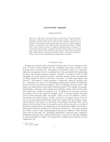
INVENTORY THEORY11Figure 4. Graph of cy L(y) ([1], pg.780).If cy L(y) is drawn as a function of y, it will appear as shown in Figure 4.Now we will define S as the value of y that minimizes cy L(y), and define s asthe smallest value of y for which cs L(s) K cS L(S). From Figure 4, it canbe seen thatIf x S, then K cy L(y) cx L(x), for all y x,so thatK c(y x) L(y) L(x).The left hand side of this inequality is the expected total cost of ordering y xto bring the inventory level up to y, and the right hand side of this inequality is theexpected total cost if no ordering occurs. Therefore, the optimal policy says thatif x
Inventory models are classi ed as either deterministic or stochastic. Determin-istic models are models where the demand for a time period is known, whereas in stochastic models the demand is a random variable having a known probability dis-tribution. These models can also be classi ed by the way the inventory is reviewed,