Transcription
ChapterTenBasic Regression Analysis withTime Series DataIn this chapter, we begin to study the properties of OLS for estimating linear regressionmodels using time series data. In Section 10.1, we discuss some conceptual differences between time series and cross-sectional data. Section 10.2 provides some examples of time series regressions that are often estimated in the empirical social sciences. Wethen turn our attention to the finite sample properties of the OLS estimators and state theGauss-Markov assumptions and the classical linear model assumptions for time seriesregression. While these assumptions have features in common with those for the crosssectional case, they also have some significant differences that we will need to highlight.In addition, we return to some issues that we treated in regression with crosssectional data, such as how to use and interpret the logarithmic functional form anddummy variables. The important topics of how to incorporate trends and account forseasonality in multiple regression are taken up in Section 10.5.10.1 THE NATURE OF TIME SERIES DATAAn obvious characteristic of time series data which distinguishes it from cross-sectionaldata is that a time series data set comes with a temporal ordering. For example, inChapter 1, we briefly discussed a time series data set on employment, the minimumwage, and other economic variables for Puerto Rico. In this data set, we must know thatthe data for 1970 immediately precede the data for 1971. For analyzing time series datain the social sciences, we must recognize that the past can effect the future, but not viceversa (unlike in the Star Trek universe). To emphasize the proper ordering of time seriesdata, Table 10.1 gives a partial listing of the data on U.S. inflation and unemploymentrates in PHILLIPS.RAW.Another difference between cross-sectional and time series data is more subtle. InChapters 3 and 4, we studied statistical properties of the OLS estimators based on thenotion that samples were randomly drawn from the appropriate population.Understanding why cross-sectional data should be viewed as random outcomes is fairlystraightforward: a different sample drawn from the population will generally yield different values of the independent and dependent variables (such as education, experience, wage, and so on). Therefore, the OLS estimates computed from different randomsamples will generally differ, and this is why we consider the OLS estimators to be random variables.311
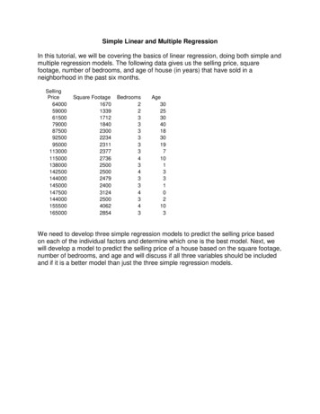
Part 2Regression Analysis with Time Series DataTable 10.1Partial Listing of Data on U.S. Inflation and Unemployment Rates, 1948–1996YearInflationUnemployment19488.13.81949 1.2 5.919501.35.319517.93.3 19942.66.119952.85.619963.05.4How should we think about randomness in time series data? Certainly, economictime series satisfy the intuitive requirements for being outcomes of random variables.For example, today we do not know what the Dow Jones Industrial Average will be atits close at the end of the next trading day. We do not know what the annual growth inoutput will be in Canada during the coming year. Since the outcomes of these variablesare not foreknown, they should clearly be viewed as random variables.Formally, a sequence of random variables indexed by time is called a stochasticprocess or a time series process. (“Stochastic” is a synonym for random.) When wecollect a time series data set, we obtain one possible outcome, or realization, of the stochastic process. We can only see a single realization, because we cannot go back in timeand start the process over again. (This is analogous to cross-sectional analysis where wecan collect only one random sample.) However, if certain conditions in history had beendifferent, we would generally obtain a different realization for the stochastic process,and this is why we think of time series data as the outcome of random variables. Theset of all possible realizations of a time series process plays the role of the populationin cross-sectional analysis.10.2 EXAMPLES OF TIME SERIES REGRESSION MODELSIn this section, we discuss two examples of time series models that have been useful inempirical time series analysis and that are easily estimated by ordinary least squares.We will study additional models in Chapter 11.312
Chapter 10Basic Regression Analysis with Time Series DataStatic ModelsSuppose that we have time series data available on two variables, say y and z, where ytand zt are dated contemporaneously. A static model relating y to z isyt 0 1zt ut , t 1,2, , n.(10.1)The name “static model” comes from the fact that we are modeling a contemporaneousrelationship between y and z. Usually, a static model is postulated when a change in zat time t is believed to have an immediate effect on y: yt 1 zt , when ut 0. Staticregression models are also used when we are interested in knowing the tradeoff betweeny and z.An example of a static model is the static Phillips curve, given byinft 0 1unemt ut ,(10.2)where inft is the annual inflation rate and unemt is the unemployment rate. This form ofthe Phillips curve assumes a constant natural rate of unemployment and constant inflationary expectations, and it can be used to study the contemporaneous tradeoff betweenthem. [See, for example, Mankiw (1994, Section 11.2).]Naturally, we can have several explanatory variables in a static regression model.Let mrdrtet denote the murders per 10,000 people in a particular city during year t, letconvrtet denote the murder conviction rate, let unemt be the local unemployment rate,and let yngmlet be the fraction of the population consisting of males between the agesof 18 and 25. Then, a static multiple regression model explaining murder rates ismrdrtet 0 1convrtet 2unemt 3yngmlet ut .(10.3)Using a model such as this, we can hope to estimate, for example, the ceteris paribuseffect of an increase in the conviction rate on criminal activity.Finite Distributed Lag ModelsIn a finite distributed lag (FDL) model, we allow one or more variables to affect ywith a lag. For example, for annual observations, consider the modelgfrt 0 0pet 1pet 1 2pet 2 ut ,(10.4)where gfrt is the general fertility rate (children born per 1,000 women of childbearingage) and pet is the real dollar value of the personal tax exemption. The idea is to seewhether, in the aggregate, the decision to have children is linked to the tax value of having a child. Equation (10.4) recognizes that, for both biological and behavioral reasons,decisions to have children would not immediately result from changes in the personalexemption.Equation (10.4) is an example of the modelyt 0 z 0 tz1 t 1 z2 t 2 ut ,(10.5)313
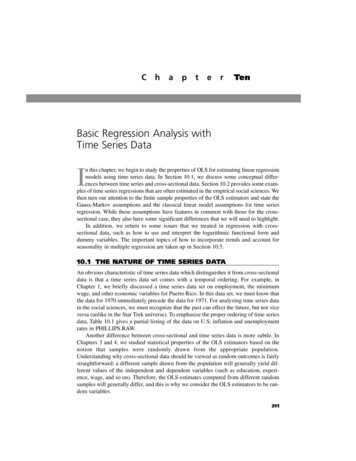
Part 2Regression Analysis with Time Series Datawhich is an FDL of order two. To interpret the coefficients in (10.5), suppose that z isa constant, equal to c, in all time periods before time t. At time t, z increases by one unitto c 1 and then reverts to its previous level at time t 1. (That is, the increase in z istemporary.) More precisely, , zt 2 c, zt 1 c, zt c 1, zt 1 c, zt 2 c, .To focus on the ceteris paribus effect of z on y, we set the error term in each timeperiod to zero. Then,yt 1 0 yt 0 c 0c 1(c 1) c 0yt 1 0 0yt 2 0 0c 1c 1yt 3 0 c,2c,12(c 1) c c 0c,2(c 1),2c 1c,2and so on. From the first two equations, yt yt 1 0, which shows that 0 is theimmediate change in y due to the one-unit increase in z at time t. 0 is usually called theimpact propensity or impact multiplier.Similarly, 1 yt 1 yt 1 is the change in y one period after the temporary change,and 2 yt 2 yt 1 is the change in y two periods after the change. At time t 3, yhas reverted back to its initial level: yt 3 yt 1. This is because we have assumed thatonly two lags of z appear in (10.5). When we graph the j as a function of j, we obtainthe lag distribution, which summarizes the dynamic effect that a temporary increase inz has on y. A possible lag distribution for the FDL of order two is given in Figure 10.1.(Of course, we would never know the parameters j; instead, we will estimate the j andthen plot the estimated lag distribution.)The lag distribution in Figure 10.1 implies that the largest effect is at the first lag.The lag distribution has a useful interpretation. If we standardize the initial value of yat yt 1 0, the lag distribution traces out all subsequent values of y due to a one-unit,temporary increase in z.We are also interested in the change in y due to a permanent increase in z. Beforetime t, z equals the constant c. At time t, z increases permanently to c 1: zs c, st and zs c 1, s t. Again, setting the errors to zero, we haveyt 1 0 yt 0 yt 1 0 yt 2 0 c 0(c 1) (c 1) 0c,2c 0(c 1) 0c 11(c 1) 1(c 1) 1c,2c,2(c 1),2and so on. With the permanent increase in z, after one period, y has increased by 0 1, and after two periods, y has increased by 0 1 2. There are no further changesin y after two periods. This shows that the sum of the coefficients on current and laggedz, 0 1 2, is the long-run change in y given a permanent increase in z and is calledthe long-run propensity (LRP) or long-run multiplier. The LRP is often of interestin distributed lag models.314
Chapter 10Basic Regression Analysis with Time Series DataFigure 10.1A lag distribution with two nonzero lags. The maximum effect is at the first lag.coefficient( j)1234lagAs an example, in equation (10.4), 0 measures the immediate change in fertilitydue to a one-dollar increase in pe. As we mentioned earlier, there are reasons to believethat 0 is small, if not zero. But 1 or 2, or both, might be positive. If pe permanentlyincreases by one dollar, then, after two years, gfr will have changed by 0 1 2.This model assumes that there are no further changes after two years. Whether or notthis is actually the case is an empirical matter.A finite distributed lag model of order q is written asyt 0 z z0 t1 t 1 zq t q ut .(10.6)This contains the static model as a special case by setting 1, 2, , q equal to zero.Sometimes, a primary purpose for estimating a distributed lag model is to test whetherz has a lagged effect on y. The impact propensity is always the coefficient on the contemporaneous z, 0. Occasionally, we omit zt from (10.6), in which case the impactpropensity is zero. The lag distribution is again the j graphed as a function of j. Thelong-run propensity is the sum of all coefficients on the variables zt j:LRP 0 1 .q(10.7)315
Part 2Regression Analysis with Time Series DataBecause of the often substantial correlation in z at different lags—that is, due to multicollinearity in (10.6)—it can be difficult to obtain precise estimates of the individual j.Interestingly, even when the j cannot beprecisely estimated, we can often get goodQ U E S T I O N1 0 . 1estimates of the LRP. We will see an example later.In an equation for annual data, suppose thatWe can have more than one explanatoryintt 1.6 .48 inft .15 inft 1 .32 inft 2 ut ,variable appearing with lags, or we can addwhere int is an interest rate and inf is the inflation rate, what are thecontemporaneous variables to an FDLimpact and long-run propensities?model. For example, the average educationlevel for women of childbearing age couldbe added to (10.4), which allows us to account for changing education levels for women.A Convention About the Time IndexWhen models have lagged explanatory variables (and, as we will see in the next chapter, models with lagged y), confusion can arise concerning the treatment of initial observations. For example, if in (10.5), we assume that the equation holds, starting at t 1,then the explanatory variables for the first time period are z1, z0, and z 1. Our convention will be that these are the initial values in our sample, so that we can always startthe time index at t 1. In practice, this is not very important because regression packages automatically keep track of the observations available for estimating models withlags. But for this and the next few chapters, we need some convention concerning thefirst time period being represented by the regression equation.10.3 FINITE SAMPLE PROPERTIES OF OLS UNDERCLASSICAL ASSUMPTIONSIn this section, we give a complete listing of the finite sample, or small sample, properties of OLS under standard assumptions. We pay particular attention to how theassumptions must be altered from our cross-sectional analysis to cover time seriesregressions.Unbiasedness of OLSThe first assumption simply states that the time series process follows a model whichis linear in its parameters.A S S U M P T I O NT S . 1( L I N E A RI NP A R A M E T E R S )The stochastic process {(xt1, xt2, , xtk, yt ): t 1,2, , n} follows the linear modelyt 0 1xt1 k xtk ut ,(10.8)where {ut : t 1,2, , n} is the sequence of errors or disturbances. Here, n is the numberof observations (time periods).316
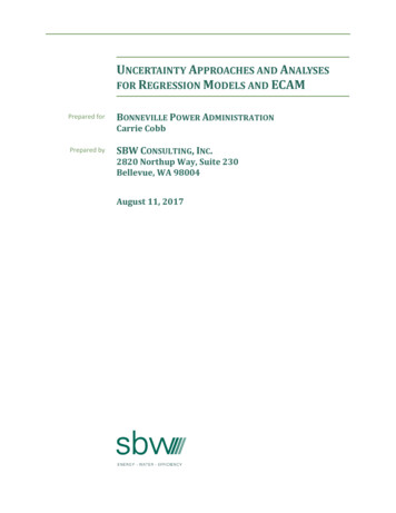
Chapter 10Basic Regression Analysis with Time Series DataTable 10.2Example of X for the Explanatory Variables in Equation 28.56.059.13In the notation xtj, t denotes the time period, and j is, as usual, a label to indicate oneof the k explanatory variables. The terminology used in cross-sectional regressionapplies here: yt is the dependent variable, explained variable, or regressand; the xtj arethe independent variables, explanatory variables, or regressors.We should think of Assumption TS.1 as being essentially the same as AssumptionMLR.1 (the first cross-sectional assumption), but we are now specifying a linear modelfor time series data. The examples covered in Section 10.2 can be cast in the form of(10.8) by appropriately defining xtj. For example, equation (10.5) is obtained by settingxt1 zt , xt2 zt 1, and xt3 zt 2.In order to state and discuss several
models using time series data. In Section 10.1, we discuss some conceptual differ-ences between time series and cross-sectional data. Section 10.2 provides some exam-ples of time series regressions that are often estimated in the empirical social sciences.We then turn our attention to the finite sample properties of the OLS estimators and state the Gauss-Markov assumptions and the classical .