Transcription
1194. Autoregressive, MA and ARMA processes4.1 Autoregressive processesOutline: Introduction The first-order autoregressive process, AR(1) The AR(2) process The general autoregressive process AR(p) The partial autocorrelation functionRecommended readings:B Chapter 4 of D. Peña (2008).B Chapter 2 of P.J. Brockwell and R.A. Davis (1996).B Chapter 3 of J.D. Hamilton (1994).Time series analysis - Module 1Andrés M. Alonso
120IntroductionB In this section we will begin our study of models for stationary processeswhich are useful in representing the dependency of the values of a time serieson its past.B The simplest family of these models are the autoregressive, which generalizethe idea of regression to represent the linear dependence between a dependentvariable y (zt) and an explanatory variable x (zt 1), using the relation:zt c bzt 1 atwhere c and b are constants to be determined and at are i.i.d N (0, σ 2). Aboverelation define the first order autoregressive process.B This linear dependence can be generalized so that the present value ofthe series, zt, depends not only on zt 1, but also on the previous p lags,zt 2, ., zt p. Thus, an autoregressive process of order p is obtained.Time series analysis - Module 1
121The first-order autoregressive process, AR(1)B We say that a series zt follows a first order autoregressive process, orAR(1), if it has been generated by:zt c φzt 1 at(33)where c and 1 φ 1 are constants and at is a white noise process withvariance σ 2. The variables at, which represent the new information that isadded to the process at each instant, are known as innovations.Example 36. We will consider zt as the quantity of water at the end ofthe month in a reservoir. During the month, c at amount of water comesinto the reservoir, where c is the average quantity that enters and at is theinnovation, a random variable of zero mean and constant variance that causesthis quantity to vary from one period to the next.If a fixed proportion of the initial amount is used up each month, (1 φ)zt 1,and a proportion, φzt 1 , is maintained the quantity of water in the reservoirat the end of the month will follow process (33).Time series analysis - Module 1
122The first-order autoregressive process, AR(1)B The condition 1 φ 1 is necessary for the process to be stationary.To prove this, let us assume that the process begins with z0 h, with hbeing any fixed value. The following value will be z1 c φh a1, the next,z2 c φz1 a2 c φ(c φh a1) a2 and, substituting successively, wecan write:z1 c φh a1z2 c(1 φ) φ2h φa1 a2z3 c(1 φ φ2) φ3h φ2a1 φa2 a3.Pt 1 iPt 1 itzt c i 0 φ φ h i 0 φ at iIf we calculate the expectation of zt, as E[at] 0,Xt 1E [zt] cφi φth.i 0For the process to be stationary it is a necessary condition that this functiondoes not depend on t.Time series analysis - Module 1
123The first-order autoregressive process, AR(1)B The mean is constant if both summands are, which requires that onincreasing t the first term converges to a constant andsecond is canceled.Pthet 1Both conditions are verified if φ 1 , because then i 0 φi is the sum of angeometric progression with ratio φ and converges to c/(1 φ), and the termφt converges to zero, thus the sum converges to the constant c/(1 φ).B With this condition, after an initial transition period, when t , all thevariables zt will have the same expectation, µ c/(1 φ), independent of theinitial conditions.B We also observe that in this process the innovation at is uncorrelated withthe previous values of the process, zt k for positive k since zt k depends onthe values of the innovations up to that time, a1, ., at k , but not on futurevalues. Since the innovation is a white noise process, its future values areuncorrelated with past ones and, therefore, with previous values of the process,zt k .Time series analysis - Module 1
124The first-order autoregressive process, AR(1)B The AR(1) process can be written using the notation of the lag operator,B, defined byBzt zt 1.(34)Letting zet zt µ and since Bezt zet 1 we have:(1 φB)ezt at.(35)B This condition indicates that a series follows an AR(1) process if on applyingthe operator (1 φB) a white noise process is obtained.B The operator (1 φB) can be interpreted as a filter that when applied tothe series converts it into a series with no information, a white noise process.Time series analysis - Module 1
125The first-order autoregressive process, AR(1)B If we consider the operator as an equation, in B the coefficient φ is calledthe factor of the equation.B The stationarity condition is that this factor be less than the unit in absolutevalue.B Alternatively, we can talk about the root of the equation of the operator,which is obtained by making the operator equal to zero and solving the equationwith B as an unknown;1 φB 0which yields B 1/φ.B The condition of stationarity is then that the root of the operator be greaterthan one in absolute value.Time series analysis - Module 1
126The first-order autoregressive process, AR(1)ExpectationB Taking expectations in (33) assuming φ 1, such that E [zt] E[zt 1] µ, we obtainµ c φµThen, the expectation (or mean) isµ c1 φ(36)Replacing c in (33) with µ(1 φ), the process can be written in deviations tothe mean:zt µ φ (zt 1 µ) atand letting zet zt µ,zet φezt 1 at(37)which is the most often used equation of the AR(1).Time series analysis - Module 1
127The first-order autoregressive process, AR(1)VarianceB The variance of the process is obtained by squaring the expression (37) andtaking expectations, which gives us:2E(ezt2) φ2E(ezt 1) 2φE(ezt 1at) E(a2t ).We let σz2 be the variance of the stationary process. The second term of thisexpression is zero, since as zet 1 and at are independent and both variableshave null expectation. The third is the variance of the innovation, σ 2, and weconclude that:σz2 φ2σz2 σ 2,from which we find that the variance of the process is:σ22σz .21 φ(38)Note that in this equation the condition φ 1 appears, so that σz2 is finiteand positive.Time series analysis - Module 1
128The first-order autoregressive process, AR(1)B It is important to differentiate the marginal distribution of a variable fromthe conditional distribution of this variable in the previous value. The marginaldistribution of each observation is the same, since the process is stationary: ithas mean µ and variance σz2. Nevertheless, the conditional distribution of zt ifwe know the previous value, zt 1, has a conditional mean:E(zt zt 1) c φzt 1and variance σ 2, which according to (38), is always less than σz2.B If we know zt 1 it reduces the uncertainty in the estimation of zt, and thisreduction is greater when φ2 is greater.B If the AR parameter is close to one, the reduction of the variance obtainedfrom knowledge of zt 1 can be very important.Time series analysis - Module 1
129The first-order autoregressive process, AR(1)Autocovariance functionB Using (37), multiplying by zt k and taking expectations gives us γk , thecovariance between observations separated by k periods, or the autocovarianceof order k:γk E [(zt k µ) (zt µ)] E [ezt k (φezt 1 at)]and as E [ezt k at] 0, since the innovations are uncorrelated with the pastvalues of the series, we have the following recursion:γk φγk 1k 1, 2, .(39)where γ0 σz2.B This equation shows that since φ 1 the dependence between observationsdecreases when the lag increases.B In particular, using (38):Time series analysis - Module 1
130φσ 2γ1 1 φ2Time series analysis - Module 1(40)
131The first-order autoregressive process, AR(1)Autocorrelation function, ACFB Autocorrelations contain the same information as the autocovariances, withthe advantage of not depending on the units of measurement. From hereon we will use the term simple autocorrelation function (ACF) to denote theautocorrelation function of the process in order to differentiate it from otherfunctions linked to the autocorrelation that are defined at the end of thissection.B Let ρk be the autocorrelation of order k, defined by: ρk γk /γ0, using(39), we have:ρk φγk 1/γ0 φρk 1.Since, according to (38) and (40), ρ1 φ, we conclude that:ρk φkand when k is large, ρk goes to zero at a rate that depends on φ.Time series analysis - Module 1(41)
132The first-order autoregressive process, AR(1)Autocorrelation function, ACFB The expression (41) shows that the autocorrelation function of an AR(1)process is equal to the powers of the AR parameter of the process and decreasesgeometrically to zero.B If the parameter is positive the linear dependence of the present on pastvalues is always positive, whereas if the parameter is negative this dependenceis positive for even lags and negative for odd ones.B When the parameter is positive the value at t is similar to the value at t 1,due to the positive dependence, thus the graph of the series evolves smoothly.Whereas, when the parameter is negative the value at t is, in general, theopposite sign of that at t 1, thus the graph shows many changes of signs.Time series analysis - Module 1
133Autocorrelation function - ExampleParameter, φ -0.5Parameter, φ -0.531Sample eter, φ 0.71520Parameter, φ 0.71Sample Autocorrelation420-2-410Lag050Time series analysis - Module 11001502000.50-0.5510Lag1520
134Representation of an AR(1) processas a sum of innovationsB The AR(1) process can be expressed as a function of the past values of theinnovations. This representation is useful because it reveals certain propertiesof the process. Using zet 1 in the expression (37) as a function of zet 2, wehavezet φ(φezt 2 at 1) at at φat 1 φ2zet 2.If we now replace zet 2 with its expression as a function of zet 3, we obtainzet at φat 1 φ2at 2 φ3zet 2and repeatedly applying this substitution gives us:zet at φat 1 φ2at 2 . φt 1a1 φtze1B If we assume t to be large, since φt will be close to zero we can representthe series as a function of all the past innovations, with weights that decreasegeometrically.Time series analysis - Module 1
135Representation of an AR(1) processas a sum of innovationsB Other possibility is to assume that the series starts in the infinite past:X zet φj at jj 0and this representation is denoted as the infinite order moving average, MA( ),of the process.B Observe that the coefficients of the innovations are precisely the coefficientsof the simple autocorrelation function.B The expression MA( ) can also be obtained directly by multiplying theequation (35) by the operator (1 φB) 1 1 φB φ2B 2 . . . , thusobtaining:zet (1 φB) 1at at φat 1 φ2at 2 . . .Time series analysis - Module 1
136Representation of an AR(1) processas a sum of innovations - ExampleExample 37. The figures show the monthly series of relative changes in theannual interest rate, defined by zt log(yt/yt 1) and the ACF. The ACcoefficients decrease with the lag: the first is of order .4, the second close to.42 .16, the third is a similar value and the rest are small and not significant.150.8.050.6Sample Autocorrelation.10.00-.050.40.2-.100-.1588 89 90 91 92 93 94 95 96 97 98 99 00 01Relative changes in the annual interest rates, Spain-0.212345678910LagDatafile interestrates.wf1Time series analysis - Module 1
137The AR(2) processB The dependency between present and past values which an AR(1) establishescan be generalized allowing zt to be linearly dependent not only on zt 1 butalso on zt 2. Thus the second order autoregressive, or AR(2) is obtained:zt c φ1zt 1 φ2zt 2 at(42)where c, φ1 and φ2 are now constants and at is a white noise process withvariance σ 2.B We are going to find the conditions that must verify the parameters for theprocess to be stationary. Taking expectations in (42) and imposing that themean be constant, results in:µ c φ1µ φ2µc,(43)1 φ1 φ2and the condition for the process to have a finite mean is that 1 φ1 φ2 6 0.which impliesTime series analysis - Module 1µ
138The AR(2) processB Replacing c with µ(1 φ1 φ2) and letting zet zt µ be the process ofdeviations to the mean, the AR(2) process is:zet φ1zet 1 φ2zet 2 at.(44)B In order to study the properties of the process it is advisable to use theoperator notations. Introducing the lag operator, B, the equation of thisprocess is:(1 φ1B φ2B 2)ezt at.(45)B The operator (1 φ1B φ2B 2) can always be expressed as (1 G1B)(1 G2B), where G 1and G 1are the roots of the equation of the operator12considering B as a variable and solving1 φ1B φ2B 2 0.Time series analysis - Module 1(46)
139The AR(2) processB The equation (46) is called the characteristic equation of the operator.B G1 and G2 are also said to be factors of the characteristic polynomial of theprocess. These roots can be real or complex conjugates.B It can be proved that the condition of stationarity is that Gi 1 , i 1, 2.B This condition is analogous to that studied for the AR(1).B Note that this result is consistent with the condition found for the mean tobe finite. If the equation1 φ1B φ2B 2 0has a unit root it is verified that 1 φ1 φ2 0 and the process is notstationary, since it does not have a finite mean.Time series analysis - Module 1
140The AR(2) processAutocovariance functionB Squaring expression (44) and taking expectations, we find that the variancemust satisfy:γ0 φ21γ0 φ22γ0 2φ1φ2γ1 σ 2.(47)B In order to calculate the autocovariance, multiplying the equation (44) byzet k and taking expectations, we obtain:γk φ1γk 1 φ2γk 2.k 1(48)B Specifying this equation for k 1, since γ 1 γ1, we haveγ1 φ1γ0 φ2γ1,which provides γ1 φ1γ0/(1 φ2). Using this expression in (47) results in theformula for the variance:(1 φ2
B Chapter 3 of J.D. Hamilton (1994). Time series analysis - Module 1 Andr es M. Alonso. 120 Introduction B In this section we will begin our study of models for stationary processes which are useful in representing the dependency of the values of a time series on its past. B The simplest family of these models are the autoregressive, which generalize the idea of regression to represent the .