Transcription
Data Preparation &Descriptive Statistics(ver. 2.7)Oscar Torres-ReynaData s.princeton.edu/training/
Basic definitions For statistical analysis we think of data as a collection of different piecesof information or facts. These pieces of information are called variables.A variable is an identifiable piece of data containing one or more values.Those values can take the form of a number or text (which could beconverted into number)In the table below variables var1 thru var5 are a collection of sevenvalues, ‘id’ is the identifier for each observation. This dataset hasinformation for seven cases (in this case people, but could also bestates, countries, etc) grouped into five 1590.850.23YesFemale77.5954.940.42YesMale
Data structure For data analysis your data should have variables as columns andobservations as rows. The first row should have the column headings.Make sure your dataset has at least one identifier (for example,individual id, family id, emale77.5954.940.42YesMaleAt least one identifierCross-sectional time series dataor panel dataFirst row should have the variable namesCross-sectional dataGroup 1Group 2Group 69.20.76NOTE: See: ssdat.php
Data format (ASCII) ASCII (American Standard Code for Information Interchange). The mostuniversally accepted format. Practically any statistical software can open/readthese type of files. Available formats: Delimited. Data is separated by comma, tab or space. The mostcommon extension is *.csv (comma-separated value). Another type ofextensions are *.txt for tab-separated data and *.prn for space-separateddata. Any statistical package can read these formats. Record form (or fixed). Data is structured by fixed blocks (for example,var1 in columns 1 to 5, var2 in column 6 to 8, etc). You will need acodebook and to write a program (either in Stata, SPSS or SAS) to readthe data. Extensions for the datasets could be *.dat, *.txt. For data in thisformat no column headings is available.PU/DSS/OTR
Data formats (comma-separated) Comma-separated value (*.csv)PU/DSS/OTR
Data format (tab/space separated) Tab separatedvalue (*.txt)Space separatedvalue (*.prn)PU/DSS/OTR
Data format (record/fixed) Record form (fixed) ASCII (*.txt, *.dat). For this format you need a codebook to figure out thelayout of the data (it indicates where a variable starts and where it ends). See next slide foran example. Notice that fixed datasets do not have column headings.PU/DSS/OTR
Codebook (ASCII to Stata using infix)NOTE: The following is a small example of a codebook. Codebooks are like maps to help youfigure out the structure of the data. Codebooks differ on how they present the layout of the data,in general, you need to look for: variable name, start column, end column or length, and formatof the variable (whether is numeric and how many decimals (identified with letter ‘F’) or whetheris a string variable marked with letter ‘A’ )Data 124263244EndFormat725273345F7.2F2.0A2F2.0A2In Stata you write the following to open the dataset.In the command window type:infix var1 1-7 var2 24-25 str2 var3 2627 var4 32-33 str2 var5 44-45 usingmydata.datNotice the ‘str#’ before var3 and var5, this is to indicate that these variables are string (text). Thenumber in str refers to the length of the variable.If you get an error like cannot be read as a number for click herePU/DSS/OTR
From ASCII to Stata using a dictionary file/infileUsing notepad or the do-file editor type:dictionary using c:\data\mydata.dat {column(1)var1%7.2fcolumn(24)var2%2fcolumn(26) str2 var3%2scolumn(32)var4%2fcolumn(44) str2 var5%2s}" Label" Label" Label" Label" Labelforforforforforvar1 "var2 "var3 "var4 "var5 "/*Do not forget to close the brackets and press enter after the last bracket*/Notice that the numbers in column(#) refers to the position where the variable starts basedon what the codebook shows. The option ‘str#’ indicates that the variable is a string (text oralphanumeric) with two characters, here you need to specify the length of the variable for Statato read it correctly.Save it as mydata.dctTo read data using the dictionary we need to import the data by using the command infile. Ifyou want to use the menu go to File – Import - “ASCII data in fixed format with a data dictionary”.With infile we run the dictionary by typing:infile using c:\data\mydataPU/DSS/OTRNOTE: Stata commands sometimes do not work with copy-and-paste. If you get error try re-typing the commandsIf you get an error like cannot be read as a number for click here
From ASCII to Stata using a dictionary file/infile (data with more than one record)If your data is in more than one records using notepad or the do-file editor type:dictionary using c:\data\mydata.dat {lines(2)line(1)column(1)var1%7.2f" Label for var1 "column(24)var2%2f" Label for var2 "line(2)column(26) str2 var3%2s" Label for var3 "column(32)var4%2f" Label for var4 "column(44) str2 var5%2s" Label for var5 "}/*Do not forget to close the brackets and press enter after the last bracket*/Notice that the numbers in column(#) refers to the position where the variable starts based on what thecodebook shows.Save it as mydata.dctTo read data using the dictionary we need to import the data by using the command infile. If you want touse the menu go to File – Import - “ASCII data in fixed format with a data dictionary”.With infile we run the dictionary by typing:infile using c:\data\mydataNOTE: Stata commands sometimes do not work with copy-and-paste. If you get error try re-typing the commandsFor more info on data with records see ta write.htmlPU/DSS/OTRIf you get an error like cannot be read as a number for click here
From ASCII to Stata: error messageIf running infix or infile you get errors like:‘1-1001-' cannot be read as a number for var1[14]‘de111' cannot be read as a number for var2[11]‘xvet-' cannot be read as a number for var3[15]‘0---0' cannot be read as a number for var4[16]‘A5' cannot be read as a number for var5[16]Make sure you specified those variables to be read as strings (str) and set to the correct length(str#), see the codebook for these.Double-check the data locations from the codebook. If the data file has more than one recordmake sure is indicated in the dictionary file.If after checking for the codebook you find no error in the data locations or the data type, thendepending of the type of variable, this may or may not be an error. Stata will still read thevariables but those non-numeric observations will be set to missing.PU/DSS/OTR
From ASCII to SPSSUsing the syntax editor in SPSS and following the data layout described in the codebook, type:FILE HANDLE FHAND /NAME 'C:\data\mydata.dat' /LRECL 1003.DATA LIST FILE FHAND FIXED RECORDS 1 TABLE /var1 1-7var2 24-25var3 26-27 (A)var4 32-33var5 44-45 (A).EXECUTE.You get /LRECL from the codebook.Select the program and run it by clicking on the arrowIf you have more than one record type:FILE HANDLE FHAND /NAME 'C:\data\mydata.dat' /LRECL 1003.DATA LIST FILE FHAND FIXED RECORDS 2 TABLE/1var1 1-7var2 24-25var3 26-27 (A)/2var4 32-33var5 44-45 (A).EXECUTE.PU/DSS/OTRNotice the ‘(A)’ after var3 and var5, this is to indicate that these variables are string (text).
From SPSS/SAS to StataIf your data is already in SPSS format (*.sav) or SAS(*.sas7bcat).You canuse the command usespss to read SPSS files in Stata or the commandusesas to read SAS files.If you have a file in SAS XPORT format you can use fduse (or go to fileimport).For SPSS and SAS, you may need to install it by typingssc install usespssssc install usesasOnce installed just typeusespss using “c:\mydata.sav”usesas using “c:\mydata.sas7bcat”Type help usespss or help usesas for more details.PU/DSS/OTR
Loading data in SPSSSPSS can read/save-as many proprietary data formats, go to file-open-data or file-save asClick here toselect thevariables youwantPU/DSS/OTR
Loading data in R1.tab-delimited (*.txt), type:mydata - read.table("mydata.txt")mydata - read.table("mydata.txt", header TRUE, na.strings "-9") #Ifmissing data is coded as “-9”2. space-delimited (*.prn), type:mydata - read.table("mydata.prn")3. comma-separated value (*.csv), type:mydata - read.csv("mydata.csv")mydata - read.csv("mydata.csv", header TRUE) #With column headings4. From SPSS/Stata to R use the foreign package, type:library(foreign) # Load the foreign package.stata.data - read.dta("mydata.dta") # For Stata.spss.data - read.spss("mydata.sav", to.data.frame TRUE) # For SPSS.5. To load data in R format usemydata - load("mydata.RData")Source: pdfAlso check: http://www.ats.ucla.edu/stat/R/modules/raw data.htmPU/DSS/OTR
Other data formats FeaturesData extensionsUser interfaceData manipulationData analysisGraphicsCostProgramextensionsOutput extensionStataSPSSSASR*.dta*.sav,*.por (portable file)*.sas7bcat,*.sas#bcat,*.xpt (xport files)*.RdataProgramming/point-and-clickMostly point-and-clickProgrammingProgrammingVery strongModerateVery strongVery ersatileVery goodVery goodGoodGoodAffordable (perpetuallicenses, renew only whenupgrade)Expensive (but not need torenew until upgrade, longterm licenses)Expensive (yearlyrenewal)Open source*.do (do-files)*.sps (syntax files)*.sas*.txt (log files)*.log (text file, any wordprocessor can read it),*.smcl (formated log, onlyStata can read it).*.spo (only SPSS can readit)(various formats)*.txt (log files, anyword processorcan read)
Compress data files (*.zip, *.gz)If you have datafiles with extension *.zip, *.gz, *.rar you need file compression software toextract the datafiles. You can use Winzip, WinRAR or 7-zip among others.7-zip (http://7-zip.org/) is freeware and deals with most compressed formats.Stata allows you to unzip files from the command window.unzipfile “c:\data\mydata.zip”You can also zip file using zipfilezipfile myzip.zip mydata.dtaPU/DSS/OTR
Before you startOnce you have your data in the proper format, before you perform anyanalysis you need to explore and prepare it first:1. Make sure variables are in columns and observations in rows.2. Make sure you have all variables you need.3. Make sure there is at least one id.4. If times series make sure you have the years you want to include inyour study.5. Make sure missing data has either a blank space or a dot (‘.’)6. Make sure to make a back-up copy of your original dataset.7. Have the codebook handy.PU/DSS/OTR
Stata color-coded systemAn important step is to make sure variables are in their expected format. Numericshould be numeric and text should be text.Stata has a color-coded system for each type. Black is for numbers, red is for textor string and blue is for labeled variables.Var2 is a string variable even though yousee numbers. You can’t do any statisticalprocedure with this variable other thansimple frequenciesFor var1 a value 2 has thelabel “Fairly well”. It is still anumeric variablePU/DSS/OTRVar3 is a numeric You can do any statisticalprocedure with this variableVar4 is clearly a string variable.You can do frequencies andcrosstabulations with this butnot any statistical procedure.
Cleaning your variablesIf you are using datasets with categorical variables you need to clean them bygetting rid of the non-response categories like ‘do not know’, ‘no answer’, ‘noapplicable’, ‘not sure’, ‘refused’, etc.Usually non-response categories have higher values like 99, 999, 9999, etc (or insome cases negative values). Leaving these will bias, for example, the mean ageor your regression results as outliers.In the example below the non-response is coded as 999 and if we leave this themean age would be 80 years, removing the 999 and setting it to missing, theaverage age goes down to 54 years.This is a frequency of age, notice the 999 value for the no . tabstat age age w999In Stata you can typereplace age . if age 999orreplace age . if age 100PU/DSS/OTRstatsageage w999mean54.5880180.72615
Cleaning your variablesNo response categories not only affect the statistics of the variable, it may alsoaffect the interpretation and coefficients of the variable if we do not remove them.In the example below responses go from ‘very well’ to ‘refused’, with codes 1 to 6.Leaving the variable ‘as-is’ in a regression model will misinterpret the variable asgoing from quite positive to refused? This does not make sense. You need toclean the variable by eliminating the no response so it goes from positive tonegative. Even more, you may have to reverse the valence so the variable goesfrom negative to positive for a better/easier interpretation. tab var1. tab var1, nolabelStatus ofNat'l EcoFreq.PercentCum.Status ofNat'l EcoFreq.PercentCum.Very wellFairly wellFairly badlyVery badlyNot DSS/OTR
Cleaning your variables (using recode in Stata)First, never work with the original variable, always keep originals original.The command recode in Stata lets you create a new variable without modifying the original.recode var1 (1 4 "Very well") (2 3 "Fairly well") (3 2 "Fairly badly")(4 1 "Very badly") (else .), gen(var1 rec) label(var1 rec)Get frequencies of both variables: var1 and var1 rec to verify:. tabvar1 rec. tab var1Status ofNat'l EcoFreq.PercentCum.Very wellFairly wellFairly badlyVery badlyNot 0RECODE ofvar1 (Statusof Nat'lEco)Freq.PercentCum.Very badlyFairly badlyFairly wellVery 3100.00Total1,358100.00Now you can use var1 rec in a regression since it is an ordinal variable where higher valuesmean positive opinions. This process is useful when combining variables to create indexes.For additional help on data management, analysis and presentation please .princeton.edu/PU/DSS/OTR
Reshape wide to long (if original data in Excel)The following dataset is not ready for analysis, years are in columns and casesand variables are in rows (click here to get it). The ideal is for years and countriesto be in rows and variables (var1 and var2) in columns. We should have fourcolumns: Country, Year, var1and var2We can prepare this dataset using Stata but we need to do some changes inExcel.PU/DSS/OTRFor R please see: ts/html/reshape.html
Reshape wide to long (if original data in Excel)First, you need to add a character to the column headings so Stata can readthem. Stata does not take numbers as variable names. In this case we add an “x”to the years. In excel you do this by using the ‘replace’ function. For the 1900s wereplace “19” for “x19”, same for the 2000s (make sure to select only theheadings). See the followingPU/DSS/OTR
Reshape wide to long (if original data in Excel)We have Replace the dots “.” (or anystring character) with a blankMake sure the numbers arenumbers. Select all and formatcells as numbers.PU/DSS/OTR
Reshape wide to long (from Excel to Stata)The table should look like.Copy and paste the table from Excel to Stata. In Stata go to Data - Data EditorPU/DSS/OTRNOTE: You can save the excel file as *.csv and open it in Stata typing insheet using exceltable.csv
Reshape wide to long (summary)idx2001x2002x2003127123593118gen id norder idreshape long x , i(id) 8datex var1x var2x var3127123593118reshape long x var , i(date) j(id) strdateidx var112127131213225239311321338
Reshape (Stata, 1)Back to the example, create a unique id for each observation, type:gen id norder idTo reshape from wide to long, typereshape long x, i(id) j(year). reshape long x, i(id) j(year)(note: j 1995 1996 1997 1998 1999 2000 2001 2002 2003 2004 2005)Datawide- longNumber of obs.14Number of variables14j variable (11 values)xij variables:x1995 x1996 . x2005- - - 1545year- xWhere: long – Goes from wide to long format. x – The variables with the prefix “x” (x1960, x1961, x1962, etc.) are to be converted from wide to long. i(id) – A unique identifier for the wide format is in variable “id”. j(year) – Indicates that the suffix of “x” (x1961, x1962, x1963, ), the years, should be put in variable called“year”.NOTE: If you have more than one variable you can list them as follows:reshape long x y z, i(id) j(year)PU/DSS/OTR
Reshape wide to long (Stata, 2)The data it should look like the picture below. Notice that var1 and var2 are together inone column as variable ‘x’ (the prefix we originally had for the years). If we had onevariable we are done, in this example we have two and we need to separate them into twocolumns, var1 and var2 . Basically we need to reshape again but this time from long towide.PU/DSS/OTR
Reshape (Stata, 3)To separate var1 and var2 we need to do a little bit of work. encode variable, gen(varlabel). 00Total154100.00First we need to create a new variable with the labels of eachvariable, type. tabencode variable, gen(varlabel)varlabelVariablevarlabel, 00100.00Total154100.00Create a do-file with the labels for each variable. This comes in handy when dealing with lots of variables.label save varlabel using varname, replaceYou will notice that a file varname.do is created. label save varlabel using varname, replacefile varname.do savedOpen the do-file with the do-file editor and do the following changes - Change “label define” to “labelvariable”- Change “varlabel 1” to “x1” and“varlabel 2” to “x2”- Delete “, modify- Save the do-filePU/DSS/OTR
Reshape (Stata, 4)To separate var1 and var2 we need to reshape again, this time from long to wide. First we need tocreate another id to identify the groups (country and years), typeegenmovedropdropid2 group(country year)id2 yearidvariableReshape the data by typingreshape wide x, i(id2) j(varlabel)order id2 country year x1 x2. reshape wide x, i(id2) j(varlabel)(note: j 1 2)DataNumber of obs.Number of variablesj variable (2 values)xij variables:long- wide1545varlabel- - - 775(dropped)x- x1 x2Where:wide – Indicates long to wide format.x – The variable of interest to go from long to wide is called“data”.i(id2) – A unique identifier for the wide format is in variable “id2”.j(varlabel) – Indicates that the suffix of “data” has to be takenfrom “”varlabel” (“varlabel” has two categories: 1 –var1- and 2 –var2).PU/DSS/OTRNOTE: If “j” is not available in your dataset, you may be ableto generate one using the following command:bysort id: gen jvar nThen reshapereshape wide data, i(id) j(jvar)
Reshape (Stata, 5)Run the do-file varname.do by selecting all andclicking on the last icon, this will change the labels forx1 and x2The final dataset will look like PU/DSS/OTR
Reshape long to wide (Stata, 1)You want to go from idtimer112127131213225239311321338to reshape wide r, i(id) j(time)EXAMPLE: If you have a dataset like this one (click hereto get it), we need to change the date variable as follows:tostring month year, replacegen date year " 0" month if length(month) 1replace date year " " month if date "“drop year monthorder id datePU/DSS/OTRidr.time1r.time2r.time3127123593118
Reshape long to wide (Stata, 2)The data will look like To reshape typereshape wide return interest, i(id) j(date) str. reshape wide return interest, i(id) j(date) str(note: j 1998 11 1998 12 1999 01 1999 02 1999 03 1999 04 1999 0 5 1999 06 1999 07 1999 08 1999 09 1999 10 1999 11 1999 12 2000 01 2000 02 2000 03 2000 04 2000 05 2000 06 2000 07 2000 08 2000 09 2000 10 2000 11 2000 12 2001 01 2 001 02 2001 03 2001 04 2001 05 2001 06 2001 07 2001 08 2001 09 2001 10 2001 11 2001 12 2002 01 2002 02 2002 03 20 02 04 20 02 05 2002 06 2002 07 2002 08 2002 09 2002 10 2002 11 2002 12 2003 01 2003 02 2003 03 2003 04 2003 05 200 3 06 2003 07 2003 08 2003 09 2003 10 2003 11 2003 12 2004 01 2004 02 2004 03 2004 04 2004 05 2004 06 2004 07 2004 08 2004 09 2004 10 2004 11 2004 12 2005 01 2005 02 2005 03 2005 04 2005 05 2005 06 2005 07 2005 08 2005 09 2005 10 2005 11 2005 12 2007 01 2007 02 2007 03 2007 04 2007 05 2007 06 2007 07 2007 08 2007 09 2007 10 2007 11)Datalong- wideNumber of obs.Number of variablesj variable (97 values)xij variables:8024date- - - 25195(dropped)returninterest- - return1998 11 return1998 12 . return2007 11interest1998 11 interest1998 12 . interest2007 11Where:wide – Indicates the type of reshape, in this case from long to wide format.return interest – The variables of interest from long to wide are “return” and “interest” (prefix for the newvariables).i(id) – A unique identifier for the wide format is in variable “id”.j(date) – Indicates the suffix of “return” and “interest” taken from ”date” (notice “xij” variables:” above)PU/DSS/OTR
Reshape long to wide (Stata, 3)The variable window and the data will look likeIf you want to sort all returns and interest together, run the following commands:xpose, clear varnamesort varnamexpose, clearorder idPU/DSS/OTR
Renaming variables (using renvars)You can use the command renvars to shorten the names of the variables renvarsinterest1998 11-interest2007 11,renvarsreturn1998 11-return2007 11,presub(interest i)presub(return r)BeforeAfterNOTE: You may have to install renvars by typing:ssc install renvarsPU/DSS/OTRType help renvars for more info. Also help rename
Descriptive statistics (definitions)Descriptive statistics are a collection of measurements of two things: location andvariability.Location tells you the central value of your variable (the mean is the mostcommon measure).Variability refers to the spread of the data from the center value (i.e. variance,standard deviation).Statistics is basically the study of what causes variability in the Standard deviationMedianRange
Descriptive statistics (location) IndicatorDefinitionFormulaIn ExcelIn StataIn RLocationThe mean is the sum of the observationsdivided by the total number ofobservations. It is the most commonindicator of central tendency of a variableMeanMedianX X AVERAGE(range of cells)inFor example: AVERAGE(J2:J31)The median is another measure of central tendency.To get the median you have to order the data from lowest tohighest. The median is the number in the middle.If the number of cases is odd the median is the single value,for an even number of cases the median is the average of thetwo numbers in the middle. It is not affected by outliers. Also MEDIAN(range of cells)known as the 50th percentile.267892 6 7 8 9 10ModeThe mode refers to the most frequent, repeated or commonnumber in the dataPU/DSS/OTR MODE(range of cells)-tabstat var1,s(mean)summary(x)ormean(x)sapply(x, mean,na.rm T)- sum var1- tabstat var1, m T)- sum var1,#mediandetailtable(x)mmodes var1 (frequencytable)NOTE: For mmodes you may have to install it by typing ssc install mmodes. You can estimate all statistics inExcell using “Descriptive Statistics” in “Analysis Toolpack”. In Stata by typing all statistics in the parenthesis tabstatvar1, s(mean median). In R see http://www.ats.ucla.edu/stat/r/faq/basic desc.htm
PU/DSS/OTR
Descriptive statistics (variability) IndicatorDefinitionFormulaIn ExcelIn StataIn RVariabilityVarianceThe variance measures thedispersion of the data from themean.s2 It is the simple mean of the squareddistance from the mean.StandarddeviationRangeThe standard deviation is thesquared root of the variance.Indicates how close the data is to themean. Assuming a normaldistribution:s 68% of the values are within 1 sd(.99) 95% within 2 sd (1.96) 99% within 3 sd (2.58). (X- tabstat var1,s(variance) X )2i(n 1)- sum var1, detail (X X ) STDEV(range of- tabstat var1, s(sd)2i(n 1)Range is a measure of dispersion. It is simple thedifference between the largest and smallest value,“max” – “min”.PU/DSS/OTR VAR(range of cells) orcells)orvar(x)sapply(x, var,na.rm T)sd(x)sapply(x, sd,na.rm T)- sum var1, detail MAX(range of cells)range (max(x)- MIN( same range of tabstat var1, s(range)min(x));rangecells)NOTE: You can estimate all statistics in Excell using “Descriptive Statistics” in “Analysis Toolpack”. In Stata by typingall statistics in the parenthesis tabstat var1, s(mean median variance sd range). In R seehttp://www.ats.ucla.edu/stat/r/faq/basic desc.htm
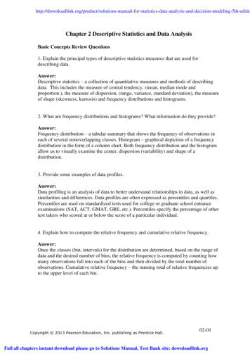
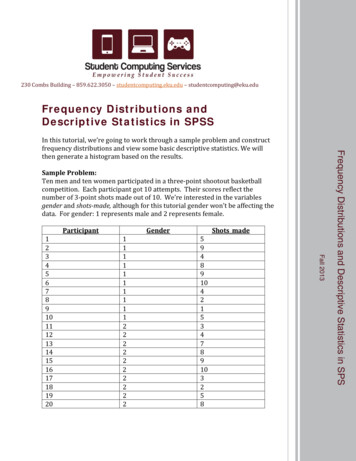
Descriptive statistics (standard deviation)1sd2sd3sd1.96sdSource: Kachigan, Sam K., Statistical Analysis. An Interdisciplinary Introduction toUnivariate & Multivariate Methods, 1986, p.61PU/DSS/OTR
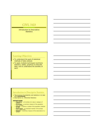
Descriptive statistics (z-scores) z-scores show how many standard deviations a single value is from themean. Having the mean is not enough.x µz iσStudentxiMean SAT scoresdz-score% xiMean SAT scoresdz-score% xiMean SAT scoresdz-score% 81620.3664.2%35.8%C222118581622.2498.7%1.3%NOTE: To get the %(below) you can use the tables at the end of any statistics book or in Excel use normsdist(z-score). %(above) is just 1-%(below).In Stata type:egen z var1 std(var1)gen below normal(z var1)gen above 1-belowPU/DSS/OTR
PU/DSS/OTR
Descriptive statistics (distribution) IndicatorDefinitionFormulaIn ExcelIn StataIn RVariabilityIndicates how close the sample mean isStandardfrom the ‘true’ population mean. Iterrorincreases as the variation increases and it(deviation)decreases as the sample size goes up. Itof the meanprovides a measure of uncertainty.ConfidenceThe range where the 'true' value of theintervals formean is likely to fall most of the timethe meanSE X σsem sd(x)/sqrt (STDEV(range oftabstat eme range of cells))).nUse “Descriptive Statistics”in the “Data Analysis” tab ci var1CI X X SE X * Z(1)Use package“pastecs”DistributionMeasures the symmetry of the distribution(whether the mean is at the center of thedistribution). The skewness value of anormal distribution is 0. A negative valueSkewnessSk indicates a skew to the left (left tail islonger that the right tail) and a positivevalues indicates a skew to the right (righttail is longer than the left one)Measures the peakedness (or flatness) ofa distribution. A normal distribution has avalue of 3. A kurtosis 3 indicates a sharpKurtosisK peak with heavy tails closer to the mean(leptokurtic ). A kurtosis 3 indicates theopposite a flat top (platykurtic).Notation:PU/DSS/OTRXi individual value of XX(bar) mean of Xn sample sizes2 variances standard deviationSEX(bar) standard error of the meanZ critical value (Z 1.96 give a 95% certainty) (X X ) SKEW(range of cells)(n 1)s 3 (X3i X ) KURT(range of cells)(n 1)s 44i-tabstat var1,Customs(skew)- sum var1, estimationdetail-tabstat var1,Customs(k)estimation- sum var1,kurtosis(x)detailFor more info check the module “Descriptive Statisticswith Excel/Stata” in http://dss.princeton.edu/training/Excel 2007 1033.aspx(1) ForFor Excel 2003 1033.aspx
Confidence intervals Confidence intervals are ranges where the true mean is expected to lie.xiMean SAT 47StudentxiMean SAT 07StudentxiMean SAT 16Studentlower(95%) (Mean SAT score) – (SE*1.96)upper(95%) (Mean SAT score) (SE*1.96)PU/DSS/OTR
Coefficient of variation (CV) Measure of dispersion, helps compare variation across variables with different units. A variable withhigher coefficient of variation is more dispersed than one with lower CV.ABB/AMeanStandard DeviationCoefficient of variation256.8727%1849275.1115%Average score (grade)8010.1113%Height (in)664.667%Newspaper readership(times/wk)51.2826%Age (years)SATCV works only with variables with positive values.PU/DSS/OTR
Examples (Excel)Click here to get the tableAgeUse “Descriptive Statistics” in the“Data Analysis” tab.MeanStandard osisSkewnessRangeMinimumMaximumSumCountAverage score(grade)SAT25.2Mean1.254325848Standard an50.22838301Standard um30CountPU/DSS/OTR For Excel 2007 1033.aspxFor Excel 2003 http://office.mic
For SPSS and SAS, you may need to install it by typing ssc install usespss ssc install usesas Once installed just type usespss using "c:\mydata.sav" usesas using "c:\mydata.sas7bcat" Type help usespss or help usesasfor more details.