WIXLIB

0.050.050.00-0.05SP5000.10 -0.15-0.05MSFT0.1510CHAPTER 1 DESCRIPTIVE STATISTICS FOR FINANCIAL DATA200020052010IndexFigure 1.5: Daily returns on Microsoft and the S&P 500 index.Figure 1.5 shows the daily simple returns on Microsoft and the S&P 500index created with plot(msftSp500DailyRetS, main "", panel my.panel, col c("black", "blue"))Compared with the monthly returns, the daily returns are closer to zeroand the magnitude of the fluctuations (volatility) is smaller. However, theclustering of periods of high and low volatility is more pronounced in the dailyreturns. As with the monthly returns, the volatility of the daily returns onMicrosoft is larger than the volatility of the S&P 500 returns. Also, thedaily returns show some large and small “spikes” that represent unusuallylarge (in absolute value) daily movements (e.g., Microsoft up 20% in one dayand down 15% on another day). The monthly returns do not exhibit suchextreme movements relative to typical volatility.

1.1 UNIVARIATE DESCRIPTIVE STATISTICS11Equity CurvesTo directly compare the investment performance of two or more assets, plotthe simple multi-period cumulative returns of each asset on the same graph.This type of graph, sometimes called an equity curve, shows how a one dollar investment amount in each asset grows over time. Better preformingassets have higher equity curves. For simple returns, the k-period returns 1Qare ( ) (1 ) and represent the growth of one dollar invested 0for periods. For continuously compounded returns, the k-period returns 1P However, this cc -period return must be converted to aare ( ) 0simple -period return, using ( ) exp ( ( )) 1 to properly representthe growth of one dollar invested for periods.Example 6 Equity curves for Microsoft and S&P 500 monthly returnsTo create the equity curves for Microsoft and the S&P 500 index based onsimple returns use: equityCurveMsft cumprod(1 msftRetS)equityCurveSp500 cumprod(1 sp500RetS)dataToPlot merge(equityCurveMsft, equityCurveSp500)plot(dataToPlot, plot.type "single", ylab "Cumulative Returns",col c("black", "blue"), lwd 2)legend(x "topright", legend c("MSFT", "SP500"),col c("black", "blue"), lwd 2)The R function cumprod() creates the cumulative products needed for theequity curves. Figure 1.6 shows that a one dollar investment in Microsoftdominated a one dollar investment in the S&P 500 index over the givenperiod. In particular, 1 invested in Microsoft grew to about 2.10 (overabout 12 years) whereas 1 invested in the S&P 500 index only grew toabout 1.40. Notice the huge increases and decreases in value of Microsoftduring the dot-com bubble and bust over the period 1998 - 2001. DrawdownsTo be completed

12CHAPTER 1 DESCRIPTIVE STATISTICS FOR FINANCIAL DATA2.01.01.5Cumulative Returns2.53.0MSFTS P5001999200120032005200720092011Ind e xFigure 1.6: Monthly cumulative continuously componded returns on Microsoft and the S&P 500 index.1.1.3Descriptive Statistics for the Distribution of ReturnsIn this section, we consider graphical and numerical descriptive statistics forthe unknown marginal pdf, ( ) of returns. Recall, we assume that theobserved sample { } 1 is a realization from a covariance stationary andergodic time series { } where each is a continuous random variable withcommon pdf ( ) The goal is to use { } 1 to describe properties of ( ) We study returns and not prices because prices are non-stationary. Sample descriptive statistics are only meaningful for covariance stationary andergodic time series.HistogramsA histogram of returns is a graphical summary used to describe the generalshape of the unknown pdf ( ) It is constructed as follows. Order returnsfrom smallest to largest. Divide the range of observed values into equally

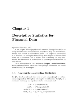
1.1 UNIVARIATE DESCRIPTIVE STATISTICS13sized bins. Show the number or fraction of observations in each bin using abar chart.Example 7 Histograms for the daily and monthly returns on Microsoft andthe S&P 500 indexFigure 1.7 shows the histograms of the daily and monthly returns on Microsoft stock and the S&P 500 index created using the R function hist(): par(mfrow c(2,2)) hist(msftRetS, main "", col "cornflowerblue") hist(msftDailyRetS, main "", col "cornflowerblue") hist(sp500RetS, main "", col "cornflowerblue") hist(sp500DailyRetS, main "", col "cornflowerblue") par(mfrow c(1,1))All histograms have a bell-shape like the normal distribution. The histogramsof daily returns are centered around zero and those for the monthly returnare centered around values slightly larger than zero. The bulk of the daily(monthly) returns for Microsoft and the S&P 500 are between -5% and 5%(-20% and 20%) and -3% and 3% (-10% and 10%), respectively. The histogram for the S&P 500 monthly returns is slightly skewed left (long lefttail) due to more large negative returns than large positive returns whereasthe histograms for the other returns are roughly symmetric.When comparing two or more return distributions, it is useful to use thesame bins for each histogram. Figure ? shows the histograms for Microsoftand S&P 500 returns using the same 15 bins, created with the R code: msftHist hist(msftRetS, plot FALSE, breaks 15) par(mfrow c(2,2)) hist(msftRetS, main "", col "cornflowerblue") hist(msftDailyRetS, main "", col "cornflowerblue", breaks msftHist breaks) hist(sp500RetS, main "", col "cornflowerblue", breaks msftHist breaks) hist(sp500DailyRetS, main "", col "cornflowerblue", breaks msftHist breaks) par(mfrow c(1,1))

140010006000 200Frequency10 20 30 40 50 600Frequency14CHAPTER 1 DESCRIPTIVE STATISTICS FOR FINANCIAL quency0Frequency0.05msftDailyRetS10 20 30 40 50 60 70m sftRetS-0.20-0.100.00s p500RetS0.10-0.10-0.050.000.050.10sp500Daily RetSFigure 1.7: Histograms of monthly continuously compounded returns on Microsoft stock and S&P 500 index.Using the same bins for all histograms allows us to see more clearly that thedistribution of monthly returns is more spread out than the distributions fordaily returns, and that the distribution of S&P 500 returns is more tightlyconcentrated around zero than the distribution of Microsoft returns. Example 8 Are Microsoft returns normally distributed? A first look.The shape of the histogram for Microsoft returns suggests that a normaldistribution might be a good candidate for the unknown distribution of Microsoft returns. To investigate this conjecture, we simulate random returnsfrom a normal distribution with mean and standard deviation calibrated tothe Microsoft daily and monthly returns using: set.seed(123) gwnDaily rnorm(length(msftDailyRetS), mean mean(msftDailyRetS),

1515001000Frequency50000Frequency10 20 30 40 50 601.1 UNIVARIATE DESCRIPTIVE y50000Frequency0.2msftDailyRetS10 20 30 40 50 60 500DailyRetSFigure 1.8: Histograms for Microsoft and S&P 500 returns using the samebins. sd sd(msftDailyRetS)) gwnDaily zoo(gwnDaily, index(msftDailyRetS)) gwnMonthly rnorm(length(msftRetS), mean mean(msftRetS), sd sd(msftRetS)) gwnMonthly zoo(gwnMonthly, index(msftRetS))Figure 1.9 shows the Microsoft monthly returns together with the simulatednormal returns created using par(mfrow c(2,2)) plot(msftRetS, main "Monthly Returns on MSFT", lwd 2, col "blue", ylim c(-0.4, 0.4)) abline(h 0)

16CHAPTER 1 DESCRIPTIVE STATISTICS FOR FINANCIAL DATA plot(gwnMonthly, main "Simulated Normal Returns", lwd 2, col "blue", ylim c(-0.4, 0.4)) abline(h 0) hist(msftRetS, main "", col "cornflowerblue", xlab "returns") hist(gwnMonthly, main "", col "cornflowerblue", xlab "returns", breaks msftHist breaks) par(mfrow c(1,1))The simulated normal returns shares many of the same features as the Microsoft returns: both fluctuate randomly about zero. However, there aresome important differences. In particular, the volatility of Microsoft returnsappears to change over time (large before 2003, small between 2003 and2008, and large again after 2008) whereas the simulated returns has constantvolatility. Additionally, the distribution of Microsoft returns has fatter tails(more extreme large and small returns) than the simulated normal returns.Apart from these features, the simulated normal returns look remarkably likethe Microsoft monthly returns.Figure 1.10 shows the Microsoft daily returns together with the simulatednormal returns. The daily returns look much less like GWN than the monthlyreturns. Here the constant volatility of simulated GWN does not matchthe volatility patterns of the Microsoft daily returns, and the tails of thehistogram for the Microsoft returns are “fatter” than the tails of the GWNhistogram. Smoothed histogramHistograms give a good visual representation of the data distribution. Theshape of the histogram, however, depends on the number of bins used. Witha small number of bins, the histogram often appears blocky and fine details ofthe distribution are not revealed. With a large number of bins, the histogrammight have many bins with very few observations. The hist() function in Rsmartly chooses the number of bins so that the resulting histogram typicallylooks good.The main drawback of the histogram as descriptive statistic for the underlying pdf of the data is that it is discontinuous. If it is believed that theunderlying pdf is continuous, it is desirable to have a continuous graphicalsummary of the pdf. The smoothed histogram achieves this goal. Given a

171.1 UNIVARIATE DESCRIPTIVE STATISTICSSimulated Normal 0.20.40.4Monthly Returns on 0 15 20 25 30 35500Frequency2005Index10 20 30 40 50 sFigure 1.9: Comparison of Microsoft monthly returns with simulated normalreturns with the same mean and standard deviation as the Microsoft returns.sample of data { } 1 the R function density() computes a smoothed estimate of the underlying pdf at each point in the bins of the histogram usingthe formula¶µ X1 ˆ ( ) 1 where (·) is a continuous smoothing function (typically a standard normaldistribution) and is a bandwidth (or bin-width) parameter that determinesthe width of the bin around in which the smoothing takes place. Theresulting pdf estimate ˆ ( ) is a two-sided weighted average of the histogramvalues around Example 9 Smoothed histogram for Microsoft monthly returns

18CHAPTER 1 DESCRIPTIVE STATISTICS FOR FINANCIAL etS0.15Simulated Normal Returns0.15Monthly Returns on 00 s0.15-0.15-0.050.050.15returnsFigure 1.10: Comparison of Microsoft daily returns with simulated normalreturns with the same mean and standard deviation as the Microsoft returns.Figure 1.11 shows the histogram of Microsoft returns overlaid with the smoothedhistogram created using MSFT.density density(msftRetS) hist(msftRetS, main "", xlab "Microsoft Monthly Returns", col "cornflowerblue", probability T, ylim c(0,5)) points(MSFT.density,type "l", col "orange", lwd 2)In Figure 1.11, the histogram is normalized (using the argument probability TRUE),so that its total area is equal to one. The smoothed density estimate transforms the blocky shape of the histogram into a smooth continuous graph.

19012Density3451.1 UNIVARIATE DESCRIPTIVE STATISTICS-0.4-0.20.00.20.4Microsoft Monthly ReturnsFigure 1.11: Histogram and smoothed density estimate for the monthly returns on Microsoft.Empirical CDFRecall, the CDF of a random variable is the function ( ) Pr( ) The empirical CDF of a data sample { } 1 is the function that counts thefraction of observations less than or equal to :1(# ) number of values sample size ̂ ( ) Example 10 Empirical CDF for daily and monthly returns on MicrosoftTo be completed

20CHAPTER 1 DESCRIPTIVE STATISTICS FOR FINANCIAL DATAEmpirical quantiles/percentilesRecall, for (0 1) the 100% quantile of the distribution of a continuous random variable with CDF is the point such that ( ) Pr( ) Accordingly, the 100% empirical quantile (or 100 percentile) of a data sample { } 1 is the data value ̂ such that · 100%of the data are less than or equal to ̂ Empirical quantiles can be easilydetermined by ordering the data from smallest to largest giving the orderedsample (also know as order statistics) (1) (2) · · · ( ) The empirical quantile ̂ is the order statistic closest to 5The empirical quartiles are the empirical quantiles for 0 25 0 5 and0 75 respectively. The second empirical quartile ̂ 50 is called the samplemedian and is the data point such that half of the data is less than or equalto its value. The interquartile range (IQR) is the difference between the 3rdand 1st quartileIQR ̂ 75 ̂ 25 and shows the size of the middle of the data distribution.Example 11 Empirical quantiles of the Microsoft and S&P 500 monthlyreturnsThe R function quantile() computes empirical quantiles for a single dataseries. By default, quantile() returns the empirical quartiles as well as theminimum and maximum values: quantile(msftRetS)0%25%50%75%100%-0.343450 -0.048561 0.008377 0.057303 0.407878 quantile(sp500RetS)0%25%50%75%100%-0.16942 -0.02094 0.00809 0.03532 0.107725There is no unique way to determine the empirical quantile from a sample of size for all values of . The R function quantile() can compute empirical quantile using oneof seven different definitions.

1.1 UNIVARIATE DESCRIPTIVE STATISTICS21The left (right) quantiles of the Microsoft monthly returns are smaller (larger)than the respective quantiles for the S&P 500 index.To compute quantiles for a specified use the probs argument. Forexample, to compute the 1% and 5% quantiles of the monthly returns use quantile(msftRetS,probs c(0.01,0.05))1%5%-0.1892 -0.1371 quantile(sp500RetS,probs c(0.01,0.05))1%5%-0.12040 -0.08184Here we see that 1% of the Microsoft cc returns are less than -18.9% and 5%of the returns are less than -13.7%, respectively. For the S&P 500 returns,these values are -12.0% and -8.2%, respectively.To compute the median and IQR values for monthly returns use the Rfunctions median() and IQR(), respectively apply(msftSp500RetS, 2, median)MSFTSP5000.008377 0.008090 apply(msftSp500RetS, 2, IQR)MSFTSP5000.10586 0.05626The median returns are similar (about 0.8% per month) but the IQR forMicrosoft is about twice as large as the IQR for the S&P 500 index. Historical/Empirical VaRRecall, the 100% value-at-risk (VaR) of an investment of is VaR where is the 100% quantile of the probability distribution ofthe investment simple rate of return The 100% historical VaR (sometimes called empirical VaR or Historical Simulation VaR) of an investmentof is defined as VaR ̂ where ̂ is the empirical quantile of a sample of simple returns { } 1 For a sample of continuously compounded returns { } 1 with empirical quantile ̂ , VaR (exp( ̂ ) 1)

22CHAPTER 1 DESCRIPTIVE STATISTICS FOR FINANCIAL DATAHistorical VaR is based on the distribution of the observed returns andnot on any assumed distribution for returns (e.g., the normal distribution).Example 12 Using empirical quantiles to compute historical Value-at-RiskConsider investing 100 000 in Microsoft and the S&P 500 over amonth. The 1% and 5% historical VaR values for these investments basedon the historical samples of monthly returns are: W 100000msftQuantiles quantile(msftRetS, probs c(0.01, 0.05))sp500Quantiles quantile(sp500RetS, probs c(0.01, 0.05))msftVaR W*msftQuantilessp500VaR W*sp500QuantilesmsftVaR1%5%-18923 -13711 sp500VaR1%5%-12040 -8184Based on the empirical distribution of the monthly returns, a 100,000 monthlyinvestment in Microsoft will lose 13,711 or more with 5% probability andwill lose 18,923 or more with 1% probability. The corresponding values forthe S&P 500 are 8,184 and 12,040, respectively. The historical VaR valuesfor the S&P 500 are considerable smaller than those for Microsoft. In thissense, investing in Microsoft is a riskier than investing in the S&P 500 index.1.1.4QQ-plotsOften it is of interest to see if a given data sample could be viewed as a randomsample from a specified probability distribution. One easy and effective wayto do this is to compare the empirical quantiles of a data sample to thosefrom a reference probability distribution. If the quantiles match up, thenthis provides strong evidence that the reference distribution is appropriatefor describing the distribution of the observed data. If the quantiles do notmatch up, then the observed differences between the empirical quantiles andthe reference quantiles can be used to determine a more appropriate reference

231.1 UNIVARIATE DESCRIPTIVE STATISTICSSP500 Monthly Returns0.10MSFT Monthly Returns0.050.00-0.05Sample oretical QuantilesGWN DailyMSFT Daily ReturnsSP500 Daily Returns0.05-0.15-0.050.00Sample Quantiles0.05-0.05-0.020.02Sample Quantiles0.150.10Theoretical Quantiles0.06Theoretical Quantiles-0.06Sample Quantiles0.0Sample Quantiles0.10.0-0.1-0.2Sample Quantiles0.20.4GWN Monthly-202Theoretical Quantiles-202Theoretical Quantiles-202Theoretical QuantilesFigure 1.12: Normal QQ-plots for GWN, Microsoft returns and S&P 500returns.distribution. It is common to use the normal distribution as the referencedistribution, but any distribution can, in principle be used.The quantile-quantile plot (QQ-plot) gives a graphical comparison of theempirical quantiles of a data sample to those from a specified reference distribution. The QQ-plot is an xy-plot with the reference distribution quantileson the x-axis and the empirical quantiles on the y-axis. If the quantiles exactly match up then the QQ-plot is a straight line. If the quantiles do notmatch up, then the shape of the QQ-plot indicates which features of the dataare not captured by the reference distribution.Example 13 No

Feb 03, 2015 · Descriptive Statistics for Financial Data Updated: February 3, 2015 In this chapter we use graphical and numerical descriptive statistics to study the distribution and dependence properties of daily and monthly asset returns on a number of representative assets. The purpose of this cha