Transcription
Basics of StatisticsJarkko Isotalo302010Std. Dev 486.32Mean 3553.8N hts of children during years 1965-69Time to Accelerate from 0 to 60 mph (sec)30201000Horsepower100200300
1PrefaceThese lecture notes have been used at Basics of Statistics course held in University of Tampere, Finland. These notes are heavily based on the followingbooks.Agresti, A. & Finlay, B., Statistical Methods for the Social Sciences, 3th Edition. Prentice Hall, 1997.Anderson, T. W. & Sclove, S. L., Introductory Statistical Analysis. Houghton Mifflin Company, 1974.Clarke, G.M. & Cooke, D., A Basic course in Statistics. Arnold,1998.Electronic Statistics ome.html.Freund, J.E.,Modern elementary statistics. Prentice-Hall, 2001.Johnson, R.A. & Bhattacharyya, G.K., Statistics: Principles andMethods, 2nd Edition. Wiley, 1992.Leppälä, R., Ohjeita tilastollisen tutkimuksen toteuttamiseksi SPSSfor Windows -ohjelmiston avulla, Tampereen yliopisto, Matematiikan, tilastotieteen ja filosofian laitos, B53, 2000.Moore, D., The Basic Practice of Statistics. Freeman, 1997.Moore, D. & McCabe G., Introduction to the Practice of Statistics, 3th Edition. Freeman, 1998.Newbold, P., Statistics for Business and Econometrics. PrenticeHall, 1995.Weiss, N.A., Introductory Statistics. Addison Wesley, 1999.Please, do yourself a favor and go find originals!
21The Nature of Statistics[Agresti & Finlay (1997), Johnson & Bhattacharyya (1992), Weiss(1999), Anderson & Sclove (1974) and Freund (2001)]1.1What is statistics?Statistics is a very broad subject, with applications in a vast number ofdifferent fields. In generally one can say that statistics is the methodologyfor collecting, analyzing, interpreting and drawing conclusions from information. Putting it in other words, statistics is the methodology which scientistsand mathematicians have developed for interpreting and drawing conclusions from collected data. Everything that deals even remotely with thecollection, processing, interpretation and presentation of data belongs to thedomain of statistics, and so does the detailed planning of that precedes allthese activities.Definition 1.1 (Statistics). Statistics consists of a body of methods for collecting and analyzing data. (Agresti & Finlay, 1997)From above, it should be clear that statistics is much more than just the tabulation of numbers and the graphical presentation of these tabulated numbers.Statistics is the science of gaining information from numerical and categorical1 data. Statistical methods can be used to find answers to the questionslike: What kind and how much data need to be collected? How should we organize and summarize the data? How can we analyse the data and draw conclusions from it? How can we assess the strength of the conclusions and evaluate theiruncertainty?1Categorical data (or qualitative data) results from descriptions, e.g. the blood typeof person, marital status or religious affiliation.
3That is, statistics provides methods for1. Design: Planning and carrying out research studies.2. Description: Summarizing and exploring data.3. Inference: Making predictions and generalizing about phenomena represented by the data.Furthermore, statistics is the science of dealing with uncertain phenomenonand events. Statistics in practice is applied successfully to study the effectiveness of medical treatments, the reaction of consumers to television advertising, the attitudes of young people toward sex and marriage, and muchmore. It’s safe to say that nowadays statistics is used in every field of science.Example 1.1 (Statistics in practice). Consider the following problems:–agricultural problem: Is new grain seed or fertilizer more productive?–medical problem: What is the right amount of dosage of drug to treatment?–political science: How accurate are the gallups and opinion polls?–economics: What will be the unemployment rate next year?–technical problem: How to improve quality of product?1.2Population and SamplePopulation and sample are two basic concepts of statistics. Population canbe characterized as the set of individual persons or objects in which an investigator is primarily interested during his or her research problem. Sometimeswanted measurements for all individuals in the population are obtained, butoften only a set of individuals of that population are observed; such a set ofindividuals constitutes a sample. This gives us the following definitions ofpopulation and sample.Definition 1.2 (Population). Population is the collection of all individualsor items under consideration in a statistical study. (Weiss, 1999)Definition 1.3 (Sample). Sample is that part of the population from whichinformation is collected. (Weiss, 1999)
4Population vs. Sample Figure 1: Population and SampleAlways only a certain, relatively few, features of individual person or objectare under investigation at the same time. Not all the properties are wantedto be measured from individuals in the population. This observation emphasize the importance of a set of measurements and thus gives us alternativedefinitions of population and sample.Definition 1.4 (Population). A (statistical) population is the set of measurements (or record of some qualitive trait) corresponding to the entire collection of units for which inferences are to be made. (Johnson & Bhattacharyya, 1992)Definition 1.5 (Sample). A sample from statistical population is the set ofmeasurements that are actually collected in the course of an investigation.(Johnson & Bhattacharyya, 1992)When population and sample is defined in a way of Johnson & Bhattacharyya,then it’s useful to define the source of each measurement as sampling unit,or simply, a unit.The population always represents the target of an investigation. We learnabout the population by sampling from the collection. There can be many
5different populations, following examples demonstrates possible discrepancieson populations.Example 1.2 (Finite population). In many cases the population under consideration is one which could be physically listed. For example:–The students of the University of Tampere,–The books in a library.Example 1.3 (Hypothetical population). Also in many cases the populationis much more abstract and may arise from the phenomenon under consideration. Consider e.g. a factory producing light bulbs. If the factory keepsusing the same equipment, raw materials and methods of production also infuture then the bulbs that will be produced in factory constitute a hypothetical population. That is, sample of light bulbs taken from current productionline can be used to make inference about qualities of light bulbs produced infuture.1.3Descriptive and Inferential StatisticsThere are two major types of statistics. The branch of statistics devotedto the summarization and description of data is called descriptive statisticsand the branch of statistics concerned with using sample data to make aninference about a population of data is called inferential statistics.Definition 1.6 (Descriptive Statistics). Descriptive statistics consist of methods for organizing and summarizing information (Weiss, 1999)Definition 1.7 (Inferential Statistics). Inferential statistics consist of methods for drawing and measuring the reliability of conclusions about populationbased on information obtained from a sample of the population. (Weiss, 1999)Descriptive statistics includes the construction of graphs, charts, and tables,and the calculation of various descriptive measures such as averages, measuresof variation, and percentiles. In fact, the most part of this course deals withdescriptive statistics.Inferential statistics includes methods like point estimation, interval estimation and hypothesis testing which are all based on probability theory.
6Example 1.4 (Descriptive and Inferential Statistics). Consider event of tossing dice. The dice is rolled 100 times and the results are forming the sampledata. Descriptive statistics is used to grouping the sample data to the following tableOutcome of the roll123456Frequencies in the sample data102018161125Inferential statistics can now be used to verify whether the dice is a fair ornot.Descriptive and inferential statistics are interrelated. It is almost always necessary to use methods of descriptive statistics to organize and summarize theinformation obtained from a sample before methods of inferential statisticscan be used to make more thorough analysis of the subject under investigation. Furthermore, the preliminary descriptive analysis of a sample oftenreveals features that lead to the choice of the appropriate inferential methodto be later used.Sometimes it is possible to collect the data from the whole population. Inthat case it is possible to perform a descriptive study on the population aswell as usually on the sample. Only when an inference is made about thepopulation based on information obtained from the sample does the studybecome inferential.1.4Parameters and StatisticsUsually the features of the population under investigation can be summarizedby numerical parameters. Hence the research problem usually becomes as oninvestigation of the values of parameters. These population parameters areunknown and sample statistics are used to make inference about them. Thatis, a statistic describes a characteristic of the sample which can then be usedto make inference about unknown parameters.
7Definition 1.8 (Parameters and Statistics). A parameter is an unknownnumerical summary of the population. A statistic is a known numerical summary of the sample which can be used to make inference about parameters.(Agresti & Finlay, 1997)So the inference about some specific unknown parameter is based on a statistic. We use known sample statistics in making inferences about unknownpopulation parameters. The primary focus of most research studies is the parameters of the population, not statistics calculated for the particular sampleselected. The sample and statistics describing it are important only insofaras they provide information about the unknown parameters.Example 1.5 (Parameters and Statistics). Consider the research problem offinding out what percentage of 18-30 year-olds are going to movies at leastonce a month. Parameter: The proportion p of 18-30 year-olds going to movies at leastonce a month. Statistic: The proportion p̂ of 18-30 year-olds going to movies at leastonce a month calculated from the sample of 18-30 year-olds.1.5Statistical data analysisThe goal of statistics is to gain understanding from data. Any data analysisshould contain following steps:
8BeginFormulate the research problemDefine population and sampleCollect the dataDo descriptive data analysisUse appropriate statistical methods to solve the research problemReport the resultsEndTo conclude this section, we can note that the major objective of statisticsis to make inferences about population from an analysis of information contained in sample data. This includes assessments of the extent of uncertaintyinvolved in these inferences.
92Variables and organization of the data[Weiss (1999), Anderson & Sclove (1974) and Freund (2001)]2.1VariablesA characteristic that varies from one person or thing to another is called avariable, i.e, a variable is any characteristic that varies from one individualmember of the population to another. Examples of variables for humans areheight, weight, number of siblings, sex, marital status, and eye color. Thefirst three of these variables yield numerical information (yield numericalmeasurements) and are examples of quantitative (or numerical) variables, last three yield non-numerical information (yield non-numerical measurements) and are examples of qualitative (or categorical) variables.Quantitative variables can be classified as either discrete or continuous.Discrete variables. Some variables, such as the numbers of children in family, the numbers of car accident on the certain road on different days, orthe numbers of students taking basics of statistics course are the results ofcounting and thus these are discrete variables. Typically, a discrete variableis a variable whose possible values are some or all of the ordinary countingnumbers like 0, 1, 2, 3, . . . . As a definition, we can say that a variable is discrete if it has only a countable number of distinct possible values. That is,a variable is is discrete if it can assume only a finite numbers of values or asmany values as there are integers.Continuous variables. Quantities such as length, weight, or temperature canin principle be measured arbitrarily accurately. There is no indivible unit.Weight may be measured to the nearest gram, but it could be measured moreaccurately, say to the tenth of a gram. Such a variable, called continuous, isintrinsically different from a discrete variable.2.1.1ScalesScales for Qualitative Variables. Besides being classified as either qualitativeor quantitative, variables can be described according to the scale on whichthey are defined. The scale of the variable gives certain structure to thevariable and also defines the meaning of the variable.
10The categories into which a qualitative variable falls may or may not havea natural ordering. For example, occupational categories have no naturalordering. If the categories of a qualitative variable are unordered, then thequalitative variable is said to be defined on a nominal scale, the wordnominal referring to the fact that the categories are merely names. If thecategories can be put in order, the scale is called an ordinal scale. Basedon what scale a qualitative variable is defined, the variable can be called asa nominal variable or an ordinal variable. Examples of ordinal variables areeducation (classified e.g. as low, high) and "strength of opinion" on someproposal (classified according to whether the individual favors the proposal,is indifferent towards it, or opposites it), and position at the end of race (first,second, etc.).Scales for Quantitative Variables. Quantitative variables, whether discreteor continuos, are defined either on an interval scale or on a ratio scale.If one can compare the differences between measurements of the variablemeaningfully, but not the ratio of the measurements, then the quantitativevariable is defined on interval scale. If, on the other hand, one can compareboth the differences between measurements of the variable and the ratio ofthe measurements meaningfully, then the quantitative variable is defined onratio scale. In order to the ratio of the measurements being meaningful,the variable must have natural meaningful absolute zero point, i.e, a ratioscale is an interval scale with a meaningful absolute zero point. For example,temperature measured on the Certigrade system is a interval variable andthe height of person is a ratio variable.2.2Organization of the dataObserving the values of the variables for one or more people or things yielddata. Each individual piece of data is called an observation and the collection of all observations for particular variables is called a data set or datamatrix. Data set are the values of variables recorded for a set of samplingunits.For ease in manipulating (recording and sorting) the values of the qualitativevariable, they are often coded by assigning numbers to the different categories, and thus converting the categorical data to numerical data in a trivialsense. For example, marital status might be coded by letting 1,2,3, and 4denote a person’s being single, married, widowed, or divorced but still coded
11data still continues to be nominal data. Coded numerical data do not shareany of the properties of the numbers we deal with ordinary arithmetic. Withrecards to the codes for marital status, we cannot write 3 1 or 2 4, andwe cannot write 2 1 4 3 or 1 3 4. This illustrates how importantit is always check whether the mathematical treatment of statistical data isreally legimatite.Data is presented in a matrix form (data matrix). All the values of particularvariable is organized to the same column; the values of variable forms thecolumn in a data matrix. Observation, i.e. measurements collected fromsampling unit, forms a row in a data matrix. Consider the situation wherethere are k numbers of variables and n numbers of observations (sample sizeis n). Then the data set should look like x11 x21 Sampling units x31 xn1Variablesx12 x13 . . .x22 x23 . . .x32 x33 . . .xn2 xn3 x1kx2k x3k . . . xnkwhere xij is a value of the j:th variable collected from i:th observation, i 1, 2, . . . , n and j 1, 2, . . . , k.
123Describing data by tables and graphs[Johnson & Bhattacharyya (1992), Weiss (1999) and Freund (2001)]3.1Qualitative variableThe number of observations that fall into particular class (or category) of thequalitative variable is called the frequency (or count) of that class. A tablelisting all classes and their frequencies is called a frequency distribution.In addition of the frequencies, we are often interested in the percentage ofa class. We find the percentage by dividing the frequency of the class bythe total number of observations and multiplying the result by 100. Thepercentage of the class, expressed as a decimal, is usually referred to as therelative frequency of the class.Relative frequency of the class Frequency in the classTotal number of observationA table listing all classes and their relative frequencies is called a relativefrequency distribution. The relative frequencies provide the most relevant information as to the pattern of the data. One should also state thesample size, which serves as an indicator of the creditability of the relativefrequencies. Relative frequencies sum to 1 (100%).A cumulative frequency (cumulative relative frequency) is obtainedby summing the frequencies (relative frequencies) of all classes up to thespecific class. In a case of qualitative variables, cumulative frequencies makessense only for ordinal variables, not for nominal variables.The qualitative data are presented graphically either as a pie chart or as ahorizontal or vertical bar graph.A pie chart is a disk divided into pie-shaped pieces proportional to the relativefrequencies of the classes. To obtain angle for any class, we multiply therelative frequencies by 360 degrees, which corresponds to the complete circle.A horizontal bar graph displays the classes on the horizontal axis and thefrequencies (or relative frequencies) of the classes on the vertical axis. Thefrequency (or relative frequency) of each class is represented by vertical bar
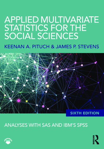
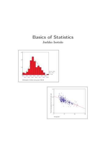
13whose height is equal to the frequency (or relative frequency) of the class.In a bar graph, its bars do not touch each other. At vertical bar graph, theclasses are displayed on the vertical axis and the frequencies of the classeson the horizontal axis.Nominal data is best displayed by pie chart and ordinal data by horizontalor vertical bar graph.Example 3.1. Let the blood types of 40 persons are as follows:O O A B A O A A A O B O B O O A O O A A A A AB A B A A O O AO O A A A O A O O ABSummarizing data in a frequency table by using SPSS:Analyze - Descriptive Statistics - Frequencies,Analyze - Custom Tables - Tables of FrequenciesTable 1: Frequency distribution of blood 6184240Graphical presentation of data in SPSS:Graphs - Interactive - Pie - Simple,Graphs - Interactive - BarPercent40.045.010.05.0100.0
145.00%n 2ABblood10.00%Bn 4OABABOPies show counts40.00%n 1645.00%n 18A40%n 2Bn 4An 18On 16bloodPercent30%AB20%10%n 16n 18OAn 4n 2BAB10%bloodFigure 2: Charts for blood types20%Percent30%40%
153.2Quantitative variableThe data of the quantitative variable can also presented by a frequency distribution. If the discrete variable can obtain only few different values, thenthe data of the discrete variable can be summarized in a same way as qualitative variables in a frequency table. In a place of the qualitative categories,we now list in a frequency table the distinct numerical measurements thatappear in the discrete data set and then count their frequencies.If the discrete variable can have a lot of different values or the quantitativevariable is the continuous variable, then the data must be grouped intoclasses (categories) before the table of frequencies can be formed. The mainsteps in a process of grouping quantitative variable into classes are:(a) Find the minimum and the maximum values variable have in the dataset(b) Choose intervals of equal length that cover the range between the minimum and the maximum without overlapping. These are called classintervals, and their end points are called class limits.(c) Count the number of observations in the data that belongs to each classinterval. The count in each class is the class frequency.(c) Calculate the relative frequencies of each class by dividing the classfrequency by the total number of observations in the data.The number in the middle of the class is called class mark of the class. Thenumber in the middle of the upper class limit of one class and the lower classlimit of the other class is called the real class limit. As a rule of thumb,it is generally satisfactory to group observed values of numerical variable ina data into 5 to 15 class intervals. A smaller number of intervals is used ifnumber of observations is relatively small; if the number of observations islarge, the number on intervals may be greater than 15.The quantitative data are usually presented graphically either as a histogram or as a horizontal or vertical bar graph. The histogram is like ahorizontal bar graph except that its bars do touch each other. The histogram is formed from grouped data, displaying either frequencies or relativefrequencies (percentages) of each class interval.
16If quantitative data is discrete with only few possible values, then the variableshould graphically be presented by a bar graph. Also if some reason it is morereasonable to obtain frequency table for quantitative variable with unequalclass intervals, then variable should graphically also be presented by a bargraph!Example 3.2. Age (in years) of 102 ,49,36,48,44Summarizing data in a frequency table by using SPSS:Analyze - Descriptive Statistics - Frequencies,Analyze - Custom Tables - Tables of FrequenciesTable 2: Frequency distribution of people’s ageFrequency distribution of people's ageValid18 - 2223 - 2728 - 3233 - 3738 - 4243 - 4748 - 5253 - 5758 - 6263 - 6768 - 72TotalFrequency61014111981212424102Graphical presentation of data in SPSS:Graphs - Interactive - Histogram,Graphs - 8.490.294.196.1100.0
7,0.07,0.07,0.08,0.06,0.07,0.06Frequency table:5Example 3.3. Prices of hotdogs ( /oz.):2.5Figure 3: Histogram for people’s 2.-2Age (in years)
18Table 3: Frequency distribution of prices of hotdogsFrequencies of prices of hotdogs ( 00.0or alternativelyTable 4: Frequency distribution of prices of hotdogs (Left Endpoints Excluded, but Right Endpoints Included)Frequencies of prices of hotdogs ( 56341154Graphical presentation of the tivePercent9.344.472.283.388.996.398.1100.0
19201000.000 - .030.060 - .090.030 - .060.120 - .150.090 - .120.180 - .210.150 - .180.240 - .270.210 - .240.270 - .300Price ( /oz)Figure 4: Histogram for pricesLet us look at another way of summarizing hotdogs’ prices in a frequencytable. First we notice that minimum price of hotdogs is 0.05. Then wemake decision of putting the observed values 0.05 and 0.06 to the same classinterval and the observed values 0.07 and 0.08 to the same class interval andso on. Then the class limits are choosen in way that they are middle valuesof 0.06 and 0.07 and so on. The following frequency table is then formed:
20Table 5: Frequency distribution of prices of hotdogsFrequencies of prices of hotdogs ( 5555555555555Figure 5: Histogram for 2.0Price ( /oz)
21Another types of graphical displays for quantitative data are(a) dotplotGraphs - Interactive - Dot(b) stem-and-leaf diagram of just stemplotAnalyze - Descriptive Statistics - Explore(c) frequency and relative-frequency polygon for frequencies and forrelative frequencies (Graphs - Interactive - Line)(d) ogives for cumulative frequencies and for cumulative relative frequencies (Graphs - Interactive - Line)3.3Sample and Population DistributionsFrequency distributions for a variable apply both to a population and to samples from that population. The first type is called the population distribution of the variable, and the second type is called a sample distribution.In a sense, the sample distribution is a blurry photograph of the populationdistribution. As the sample size increases, the sample relative frequency inany class interval gets closer to the true population relative frequency. Thus,the photograph gets clearer, and the sample distribution looks more like thepopulation distribution.When a variable is continous, one can choose class intervals in the frequencydistribution and for the histogram as narrow as desired. Now, as the samplesize increases indefinitely and the number of class intervals simultaneouslyincreases, with their width narrowing, the shape of the sample histogramgradually approaches a smooth curve. We use such curves to represent population distributions. Figure 6. shows two samples histograms, one based ona sample of size 100 and the second based on a sample of size 2000, and alsoa smooth curve representing the population distribution.
22Relative FrequencySample Distribution n 2000Relative FrequencySample Distribution n 100LowHighValues of the VariableLowHighValues of the VariableRelative FrequencyPopulation DistributionLowHighValues of the VariableFigure 6: Sample and Population DistributionsOne way to summarize a sample of population distribution is to describe itsshape. A group for which the distribution is bell-shaped is fundamentallydifferent from a group for which the distribution is U-shaped, for example.The bell-shaped and U-shaped distributions in Figure 7. are symmetric.On the other hand, a nonsymmetric distribution is said to be skewed tothe right or skewed to the left, according to which tail is longer.
23Relative FrequencyBell shapedRelative FrequencyU shapedLowHighLowValues of the VariableHighValues of the VariableFigure 7: U-shaped and Bell-shaped Frequency DistributionsRelative FrequencySkewed to the leftRelative FrequencySkewed to the rightLowHighValues of the VariableLowHighValues of the VariableFigure 8: Skewed Frequency Distributions
244Measures of center[Agresti & Finlay (1997), Johnson & Bhattacharyya (1992), Weiss(1999) and Anderson & Sclove (1974)]Descriptive measures that indicate where the center or the most typical valueof the variable lies in collected set of measurements are called measures ofcenter. Measures of center are often referred to as averages.The median and the mean apply only to quantitative data, whereas the modecan be used with either quantitative or qualitative data.4.1The ModeThe sample mode of a qualitative or a discrete quantitative variable is thatvalue of the variable which occurs with the greatest frequency in a data set.A more exact definition of the mode is given below.Definition 4.1 (Mode). Obtain the frequency of each observed value of thevariable in a data and note the greatest frequency.1. If the greatest frequency is 1 (i.e. no value occurs more than once),then the variable has no mode.2. If the greatest frequency is 2 or greater, then any value that occurs withthat greatest frequency is called a sample mode of the variable.To obtain the mode(s) of a variable, we first construct a frequency distribution for the data using classes based on single value. The mode(s) can thenbe determined easily from the frequency distribution.Example 4.1. Let us consider the frequency table for blood types of 40persons.We can see from frequency table that the mode of blood types is A.The mode in SPSS:Analyze - Descriptive Statistics - Frequencies
25Table 6: Frequency distribution of blood 6184240Percent40.045.010.05.0100.0When we measure a continuous variable (or discrete variable having a lot ofdifferent values) such as height or weight of person, all the measurements maybe different. In such a case there is no mode because every observed valuehas frequ
data. Descriptive statistics is used to grouping the sample data to the fol-lowing table Outcome of the roll Frequencies in the sample data 1 10 2 20 3 18 4 16 5 11 6 25 Inferential statistics can now be used to verify whether the dice is a fair or not. Descriptive and inferential statistics are interrelated. It is almost always nec-