WIXLIB

Commands to Generate Graphicsages 20:27;6students [2 1 4 3 2 2 0 1];figure(1); bar(ages,students)axis([19.5 27.5 0 5])xlabel(’age of students ’); ylabel(’number of students ’)figure(2); barh(ages,students)axis([0 5 19.5 27.5])ylabel(’age of students ’); xlabel(’number of students ’)52726age of studentsnumber of students43212524232221200202122232425age of students262701(a) vertical23number of students45(b) horizontalFigure 3: Bar diagramUsing the commands pie() and pie3() one can generate pie charts. With the correct optionsset labels and some of the slices can be drawn slightly removed from the pie. The result of the codebelow is shown in Figure 4.strength [55 52 36 28 13 16];Labels ��Div’}figure(1); pie(strength)figure(2); pie(strength ,[0 1 0 0 0 0],Labels)figure(3); pie3(strength a) default valuesSPFDP(b) with labelsSP(c) 3DFigure 4: Pie chartsSHA 20-12-21

Data Reduction Commands3.37Plots: stem(), stem3(), rose(), stairs()With a stem plot a vertical line with a small marker at the top can be used to visualize data. Thecode below first generates a set of random integers, and then uses a combination of unique() andhist() to determine the frequency (number of occurrences) of those numbers.ii randi(10,100,1);% generate 100 random integers between 1 and 10[anz,cent] hist(ii,unique(ii)) % count the eventsstem(cent,anz)% generate a 2D stem graphxlabel(’value ’); ylabel(’number of events ’); axis([0 11, -1 max(anz) 1])-- anz 12510121291111711cent 1234567891012584heightnumber of events610362412100.5000246value810y-0.5(a) 2D-1-1-0.510.50x(b) 3DFigure 5: Stem plotsWith stem3() a 3D stem plot can be generated.theta 0:0.2:6;stem3 (cos (theta), sin (theta), theta);xlabel(’x’); ylabel(’y’); zlabel(’height ’)MATLAB/Octave provide commands to generate angular histograms and stairstep plots.dataRaw randi([5 10],1,400);figure(1); rose(dataRaw ,8)% generate rose plottitle(’angular histogram with 8 sectors ’)[data,cent] hist(dataRaw ,unique(dataRaw))% count the eventsfigure(2); stairs(cent,data) % generate stairstep plotxlabel(’value ’); ylabel(’number of events ’);4Data Reduction CommandsIn Table 3 find a few Octave/MATLAB commands to extract information from data sets.SHA 20-12-21

Data Reduction Commands8angular histogram with 8 sectors90 8012060607030201800210number of events4015075330240656055300505270678910value(a) rose plot(b) stairs plotFigure 6: Rose plot and stairs plot4.1Commands mean(), std(), var(), median(), mode(), quantile(), boxplot() For a vector x Rn the command mean(x) determines the mean value bymean(x) x̄ n1 Xxjnj 1 For a vector x Rn the command std(x) determines the standard deviation by the formula pstd(x) var(x) 1n 1 1/2nX(xj x̄)2 j 1By default std() will normalize by (n 1), but using an option you may divide by n, e.g. byusing std(x, 1). For a vector x Rn the command var(x) determines the variance by the formulavar(x) (std(x))2 n1 X(xj x̄)2n 1j 1By default var() will normalize by (n 1), but using an option you may divide by n, e.g. byusing var(x,1). For a vector x Rn the command median(x) determines the median value. For a sortedvector is is given by(x(n 1)/2if n is oddmedian(x) 1if n is even2 (xn/2 xn/2 1 ) For a vector x Rn the command mode(x) determines the most often occurring value in x.The commands mode(randi(10,20,1)) generate 20 random integer values between 1 and 10,and then the most often generated value.SHA 20-12-21

Data Reduction Commands9mean()mean value of a data setstd()standard deviation of a data setvar()variance of a data setmedian()median value of a data setmode()determine the most frequently occurring valuequantile()determine arbitrary quantilesboxplot()generate a boxplotLinearRegression()perform a linear regressionregress()perform a linear regressionlscov()generalized least square estimation, with weightspolyfit()perform a linear regression for a polynomialols()perform an ordinary linear regressiongls()perform an generalized linear regressioncov()covariance matrixcorr()linear correlation matrixcorrcoef()correlation coefficientTable 3: Commands for data reduction With the command quantile() you can compute arbitrary quantiles. Observe that there aredifferent methods to determine the quantiles, leading to different results! Consult the built-indocumentation in Octave by calling help quantile . Often quartile (division by four) or percentiles (division by 100) have to be determined. Thecommand quantile() with a proper set of parameters does the job. You may also useprctile() to determine the values for the quartile (default) or other values for the divisions. With the command boxplot() you can generate a plot showing the median, the first andthird quartile as a box and the extreme values. Observe that there are different ways tocompute the positions of the quartiles and some implementations of boxplot() detect andmark outliers. By using an optional argument you can select which points are considered asoutliers. Consult the documentation in Octave. Boxplots can also be displayed horizontallyor vertically, as shown in Figure 7.N 10; % number of data pointsdata1 20*rand(N,1);Mean mean(data1)Median median(data1)StdDev std(data1) % uses a division by (N-1)Variance StdDev 2Variance2 mean((data1 -mean(data1)). 2) % uses a division by NVariance3 sum((data1 -mean(data1)). 2)/(N-1)figure(1); Quartile1 boxplot(data1)’% in Matlab slightly differentset(gca,’XTickLabel ’,{’ ’})% remove labels on x axisc axis axis(); axis([0.5 1.5 c axis(3:4)])figure(2); boxplot(data1 ,0,’ ’,0)% OctaveSHA 20-12-21

Data Reduction Commands10201510500(a) vertical5101520(b) horizontalFigure 7: Boxplots%boxplot(data1 ,’orientation ’,’horizontal ’) % Matlabset(gca,’YTickLabel ’,{’ ’}) % remove labels on y axisc axis axis(); axis([c axis(1:2),0.5 1.5])Quartile2 quantile(data1 ,[0 0.25 0.5 0.75 1])’Quantile10 quantile(data1 ,0:0.1:1)’data2 randi(10,[100,1]);ModalValue mode(data2) % determine the value occuring most oftenIt is possible to put multiple boxplots in one graph, and label the axis according to the data.In Figure 8 the abreviated names of weekdays are used to label the horizontal axis.% generate the random data, with some structureN 20; data zeros(N,7);for i 1:7data(:,i) 3 4*sin(i/4) randn(N,1);end%forboxplot(data);set(gca(),’xtick ’,[1:7],’xticklabel ’, a’,’Su’});4.2For vectors: cov(), corr(), corrcoef()For covariance and correlation coefficients first step is always to subtract the mean value of thecomponents from a vector, i.e. then the new mean value is zero. Covariance of two vectors x, y Rncov(x, y) n1 X(xj mean(x)) · (yj mean(y))n 11n 1j 1nX(xj yj mean(x) mean(y))j 1SHA 20-12-21

Data Reduction Commands111086420MoTuWeThFrSaSuFigure 8: Multiple boxplots in one figureBy default cov() will normalize by (n 1), but using an option you may divide by n, e.g. byusing cov(x,y,1). If x y we obtainn1 Xcov(x, x) (xj mean(x))2 var(x)n 1j 1 The correlation coefficient of two vectors x, y Rncorr(x, y) cov(x, y)std(x) · std(y)h( x mean( x)) , ( y mean( y ))ik x mean( x)k k y mean( y )kPnj 1 (x mean(x))j · (y mean(y))jPPn( j 1 (xj mean(x))2 )1/2 ( nj 1 (yj mean(y))2 )1/2Observe that if the average value of the components of both vectors are zero, then there is ageometric interpretation of the correlation coefficient as the angle between the two vectors.corr( x, y ) h x , y i cos(α)k xk k y kThis correlation coefficient can also be computed with by corrcoef(), which is currently notavailable in Octave.x linspace(0,pi/2,20)’; y sin(x);MeanValues [mean(x), mean(y)]Variances [var(x), var(y)]StandardDev [std(x), std(y)]Covariance cov(x,y)Correlation corr(x,y)-- MeanValues 0.785400.62944% generate some artificial dataSHA 20-12-21

Performing Linear n4.3 0.239220.489100.157940.97688120.109260.33055For matrices: mean(), std(), var(), median(), cov(), corr(), corrcoef()Most of the above commands can be applied to matrices. Use each column as one data vector.Assume that M RN m is a matrix of m column vectors with N values in each column. mean(M) compute the average of each column. The result is a row vector with m components. std(M) compute the standard deviation of each column. The result is a row vector with mcomponents. var(M) compute the variance of each column. The result is a row vector with m components. median(M) compute the median value of each column. The result is a row vector with mcomponents.To describe the effect of cov() and corr() the first step is to assure that the average of eachcolumn equals zero.Mm M - ones(N,1)*mean(M);Observe that this operation does not change the variance of the column vectors. cov(M) determines the m m covariance matrixcov(M ) 1Mm0 · MmN 1 The m m correlation matrix contains all correlation coefficients of the m column vectorsin the matrix M. To compute this, first make sure that the norm of each column vectorequals 1, i.e. the variance of the column vectors is normalized to 1 .Mm1 Mm / diag(sqrt(sum(Mm. 2)));Determine the m m (auto)correlation matrix corr(M) bycorr(M ) Mm10 · Mm1Observe that the diagonal entries are 1, since the each column vector correlates perfectly withitself.5Performing Linear RegressionThe method of least squares, linear or nonlinear regression is one of the most often used tools inscience and engineering. MATLAB/Octave provide multiple commands to perform these algorithms.SHA 20-12-21

Performing Linear Regression5.113Using LinearRegression()The command LinearRegression() was written by the author of these notes. For Octave the command is contained in the optimization package optim. You may downloadthe code at LinearRegression.m. The command can be used with MATLAB too, but you need a Matlab version.With this command you can apply the method of least square to fit a curve to a given set ofdata points. The curve does not have to be a linear function, but a linear combination of (almostarbitrary) functions. In the code below a straight line is adapted to some points on a curvey sin(x). Thus we try to find the optimal values for a and m such thatXχ2 (a m xj yj )2 is minimaljThe code to perform the this linear regression is given by% generate the artificial datax linspace(0,2,10)’; y sin(x);% perform the linear regression , aiming for a straight lineF [ones(size(x)),x];[p,e var ,r,p var] LinearRegression(F,y);Parameters and StandardDeviation [p sqrt(p var)]estimated std sqrt(mean(e var))-- Parameters and StandardDeviation 0.2022430.0917580.4778630.077345estimated std 0.15612The above result implies that the best fitting straight line is given byy a m x 0.202243 0.477863 xAssuming that the data is normally distributed one can show that the values of a and m normallydistributed. For this example the estimated standard deviation of a is given by 0.09 and thestandard deviation of m is 0.08. The standard deviation of the residuals rj a m xj yj isestimated by 0.16 . This is visually confirmed by Figure 9(a), generated by the following code.y reg F*p;plot(x,y,’ ’, x , y reg)With linear regression one may fit different curves to the given data. The code below generatesthe best matching parabola and the resulting Figure 9(b).% perform the linear regression , aiming for a parabolaF [ones(size(x)),x, x. 2];[p,e var ,r,p var] LinearRegression(F,y);Parameters and StandardDeviation [p sqrt(p var)]estimated std sqrt(mean(e var))y reg F*p;SHA 20-12-21

Performing Linear 11.52-0.200.5(a) straight line regression11.52(b) parabola regressionFigure 9: Results of two linear regressionsplot(x,y,’ ’, x , y reg)-- Parameters and StandardDeviation estimated std 0.019865Since the parabola is a better match for the points on the curve y sin(x) we find smaller estimatesfor the standard deviations of the parameters and residuals.It is possible perform linear regression with functions of multiple variables. The functionz p1 · 1 p2 · x p3 · ydescribes a plane in 3D space. A surface of this type is fit to a set of given points (xj , yj , zj ) bythe code below, resulting in Figure 10. The columns of the matrix F have to contain the values ofthe basis functions 1, x and y at the given data points.N 100; x 2*rand(N,1); y 3*rand(N,1); z 2 2*x- 1.5*y 0.5*randn(N,1);F [ones(size(x)), x , y];p LinearRegression(F,z)[x grid , y grid] meshgrid([0:0.1:2],[0:0.2:3]);z grid p(1) p(2)*x grid p(3)*y grid;figure(1); plot3(x,y,z,’*’)hold onmesh(x grid ,y grid ,z grid)xlabel(’x’); ylabel(’y’); zlabel(’z’);hold off-- p 1.76892.0606-1.4396Since only very few (N 100) points were used the exact parameter values p ( 2, 2, 1.5) arenote very accurately reproduced. Increasing N will lead to more accurate results for this simulation,or decrease the size of the random noise in 0.5*randn(N,1).SHA 20-12-21

Performing Linear Regression1564z20-22-43 2.51.52 1.5y11 0.50.50x0Figure 10: Result of a 3D linear regressionThe command LinearRegression() does not determine the confidence intervals for the parameters, but it returns the estimated standard deviations, resp. the variances. With these theconfidence intervals can be computed, using the Student-t distribution. To determine the CI modify the above code slightly.[p, , ,p var] LinearRegression(F,z);alpha 0.05;p CI p tinv(1-alpha/2,N-3)*[-sqrt(p var) sqrt(p var)]-- p CI 1.6944 2.2357 1.8490 2.2222-1.5869 -1.3495The result implies that the 95% confidence intervals for the parameters pi are given by 1.6944 p1 2.2357 1.8490 p2 2.2222with a confidence level of 95% . 1.5869 p3 1.34955.2Using regress()MATLAB and Octave provide the command regress() to perform linear regressions. The followingcode determines the best matching straight line to the given data points.x linspace(0,2,10)’; y sin(x);F [ones(size(x)),x];[p, p int , r, r int , stats] regress(y,F);parameters pparameter intervals p intestimated std std(r)-- parameters 0.202240.47786parameter intervals -0.0093515 0.4138380 0.2995040 0.6562220estimated std 0.14719SHA 20-12-21

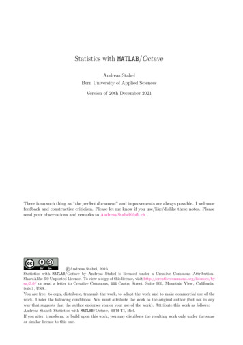
Generating Random Number16The values of the optimal parameters (obviously) have to coincide with the result generated byLinearRegression(). Instead of the standard deviations for the parameters regress() returns theconfidence intervals for the parameters. The above numbers imply for the straight line y a m x 0.0093 a 0.41380.300 m 0.656with a confidence level of 95% .The value of the confidence level can be adjusted by calling regress() with a third argument, seehelp regress .5.3Using lscov(), polyfit() or ols()The command lscov() is rather similar to the above, but can return the covariance matrix for thedetermined parameters.If your aim is to fit a polynomial to the data, you may use polyfit(). The above example fora parabola (polynomial of degree 2) is solved by[p,s] polyfit(x,y,2);p-- p -0.3863711.250604-0.026717Observe that the coefficient of the polynomial are returned in deceasing order. Since regress()and LinearRegression() are more flexible and provide more information your author’s advice isto use those, even if polyfit() would work.With Octave one may also use the command ols(), short for Ordinary Least Square. But asabove, there is no advantage over using LinearRegression().p ols(y,F)-- p -0.02671761.250604 -0.386371Generating Random NumberIn Table 4 find commands to generate random numbers, given by different distributions.As an example we generate N 1000 random numbers given by a binomial distribution withn 9 trials and p 0.8. Thus each of the 100 random number will be an integer between 0 and 9.Find the result of the code below in Figure 11 and compare with Figure 12(d), showing the resultfor the exact (non random) distribution.N 1000; data binornd(9, 0.8, N,1);% generate the random numbers[height ,centers] hist(data,unique(data)) % data for the histogrambar(centers ,height/sum(height))xlabel(’value ’); ylabel(’experimental probability ’)title(’Binomial distribution with n 9, p 0.8’)SHA 20-12-21

Commands to Work with Probability Distributions17rand()uniform distributionrandi()random integersrandn()normal distributionrande()exponentially distributedrandp()Poisson distributionrandg()gamma distributionnormrnd()normal distributionbinornd()binomial distributionexprnd()exponential distributiontrnd()Student-t distributiondiscrete rnd()discrete distributionTable 4: Commands for generating random numbersBinomial distribution with n 9, p 0.8experimental igure 11: Histogram of random numbers, generated by a binomial distribution with n 9, p 0.87Commands to Work with Probability DistributionsMATLAB/Octave provides functions to compute the values of probability density functions (PDF),and the cumulative distribution functions (CDF). In addition the inverse of the CDF are provided,i.e. solve CDF(x) y for x . As examples examine the following short code segments, using thenormal distribution. To determine the values of the PDF for a normal distribution with mean 3 and standarddeviation 2 for x values between 1 and 7 usex linspace(-1,7);plot(x,p)p normpdf(x,3,2); To determine the corresponding values of the CDF use cp normcdf(x,3,2) .

In this document a few MATLAB/Octave commands for statistics are listed and elementary sample codes are given. This should help you to get started using Octave/MATLAB for statistical problems. The