Transcription
Octave and MATLAB for EngineersAndreas Stahel, Bern University of Applied Sciences, SwitzerlandVersion of 10th September 2020
ForewordThese lecture notes were used at my school to familiarize students with Octave, to be used to solve engineering problems. A first version was based on Octave and you will still find sections to be adapted to MATLAB.The current version is avalable at AtBFH.pdf .Wherever possible I attempted to provide code working with both Octave and MATLAB . Most of thecodes are available at web.sha1.bfh.science/Labs/PWF/Codes .The notes consist of two chapters. The first chapter is an introduction to the basic Octave/MATLAB commands and data structures. Thegoal is to provide simple examples for often used commands and point out some important aspects ofprogramming in Octave or MATLAB. The students are expected to work through all of those sections.Then they should be prepared to use Octave and MATLAB for their projects. The second chapter consists of applications of MATLAB/Octave. In each section the question orproblem is formulated and then solved with the help of Octave/MATLAB. This small set of applicationswith solutions shall help you to solve your engineering problems. In class I choose a few of thosetopics and present them to the students.Starting in 2015 our students have legal access to MATLAB and thus I have to take this into account in classand most instructions and codes work with both Octave and MATLAB!There is no such thing as “the perfect lecture notes” and improvements are always possible. I welcomefeedback and constructive criticism. Please let me know if you use/like/dislike the lecture notes. Pleasesend your observations and remarks to Andreas.Stahel@bfh.ch . Andreas Stahel, 2017“Octave and Matlab for Engineers” by Andreas Stahel, BFH, Biel, Switzerland is licensed under a Creative CommonsAttribution-ShareAlike 3.0 Unported License. To view a copy of this license, visit http://creativecommons.org/licenses/bysa/3.0/ or send a letter to Creative Commons, 444 Castro Street, Suite 900, Mountain View, California, 94041, USA.You are free: to copy, distribute, transmit the work, to adapt the work and to make commercial use of the work. Underthe following conditions: You must attribute the work to the original author (but not in any way that suggests that theauthor endorses you or your use of the work). Attribute this work as follows:Andreas Stahel: Octave and Matlab for Engineers, Lecture Notes.If you alter, transform, or build upon this work, you may distribute the resulting work only under the same or similarlicense to this one.1
ContentsForeword . . . . . . . . . . . . . . . . . . . . . . . . . . . . . . . . . . . . . . . . . . . .1Introduction to Octave1.1 Starting up Octave or MATLAB and First Steps . . . . . . . . . . . . . . .1.1.1 Starting up Octave . . . . . . . . . . . . . . . . . . . . . . . . .1.1.2 Packages for Octave . . . . . . . . . . . . . . . . . . . . . . . .1.1.3 Information about the operating system and the version of Octave1.1.4 Starting up MATLAB . . . . . . . . . . . . . . . . . . . . . . . .1.1.5 Calling the operating system and using basic Unix commands . .1.1.6 How to find out whether you are working with MATLAB or Octave1.1.7 Where and how to get help . . . . . . . . . . . . . . . . . . . . .1.1.8 Vectors and matrices . . . . . . . . . . . . . . . . . . . . . . . .1.1.9 Broadcasting . . . . . . . . . . . . . . . . . . . . . . . . . . . .1.1.10 Timing of code and using a profiler . . . . . . . . . . . . . . . .1.1.11 Debugging your code . . . . . . . . . . . . . . . . . . . . . . . .1.1.12 Command line, script files and function files . . . . . . . . . . .1.1.13 Local and global variables, nested functions . . . . . . . . . . . .1.1.14 Elementary graphics . . . . . . . . . . . . . . . . . . . . . . . .1.1.15 A breaking needle ploblem . . . . . . . . . . . . . . . . . . . . .1.1.16 Exercises . . . . . . . . . . . . . . . . . . . . . . . . . . . . . .1.2 Programming with Octave . . . . . . . . . . . . . . . . . . . . . . . . .1.2.1 Displaying results and commenting code . . . . . . . . . . . . .1.2.2 Basic data types . . . . . . . . . . . . . . . . . . . . . . . . . . .1.2.3 Structured data types and arrays of matrices . . . . . . . . . . . .1.2.4 Built-in functions . . . . . . . . . . . . . . . . . . . . . . . . . .1.2.5 Working with source code . . . . . . . . . . . . . . . . . . . . .1.2.6 Loops and other control statements . . . . . . . . . . . . . . . .1.2.7 Conditions and selecting elements . . . . . . . . . . . . . . . . .1.2.8 Reading from and writing data to files . . . . . . . . . . . . . . .1.3 Solving Equations . . . . . . . . . . . . . . . . . . . . . . . . . . . . . .1.3.1 Systems of linear equations . . . . . . . . . . . . . . . . . . . .1.3.2 Zeros of polynomials . . . . . . . . . . . . . . . . . . . . . . . .1.3.3 Nonlinear equations . . . . . . . . . . . . . . . . . . . . . . . .1.3.4 Optimization . . . . . . . . . . . . . . . . . . . . . . . . . . . .1.4 Basic Graphics . . . . . . . . . . . . . . . . . . . . . . . . . . . . . . .1.4.1 2-D plots . . . . . . . . . . . . . . . . . . . . . . . . . . . . . .1.4.2 Printing figures to files . . . . . . . . . . . . . . . . . . . . . . .1.4.3 Generating histograms . . . . . . . . . . . . . . . . . . . . . . .1.4.4 Generating 3-D graphics . . . . . . . . . . . . . . . . . . . . . .1.4.5 Generating vector fields . . . . . . . . . . . . . . . . . . . . . .1.5 Basic Image Processing . . . . . . . . . . . . . . . . . . . . . . . . . . 05355606069697579798688899598
ations of Octave2.1 Numerical Integration and Magnetic Fields . . . . . . . . . . . . . . . . . . . . . . .2.1.1 Basic integration methods . . . . . . . . . . . . . . . . . . . . . . . . . . . .2.1.2 Comparison of integration commands in Octave . . . . . . . . . . . . . . . .2.1.3 From Biot–Savart to magnetic fields . . . . . . . . . . . . . . . . . . . . . . .2.1.4 Field along the central axis and the Helmholtz configuration . . . . . . . . . .2.1.5 Field in the plane of the conductor . . . . . . . . . . . . . . . . . . . . . . . .2.1.6 Field in the xz–plane . . . . . . . . . . . . . . . . . . . . . . . . . . . . . . .2.1.7 The Helmholtz configuration . . . . . . . . . . . . . . . . . . . . . . . . . . .2.1.8 List of codes and data files . . . . . . . . . . . . . . . . . . . . . . . . . . . .2.2 Linear and Nonlinear Regression . . . . . . . . . . . . . . . . . . . . . . . . . . . . .2.2.1 Linear regression for a straight line . . . . . . . . . . . . . . . . . . . . . . .2.2.2 General linear regression, matrix notation . . . . . . . . . . . . . . . . . . . .2.2.3 Estimation of the variance of parameters, confidence intervals . . . . . . . . .2.2.4 Estimation of variance of the dependent variable . . . . . . . . . . . . . . . .2.2.5 Example 1: Intensity of light of an LED depending on the angle of observation2.2.6 QR factorization and linear regression . . . . . . . . . . . . . . . . . . . . . .2.2.7 Weighted linear regression . . . . . . . . . . . . . . . . . . . . . . . . . . . .2.2.8 More commands for regression with Octave or MATLAB . . . . . . . . . . . .2.2.9 Code for the function LinearRegression() . . . . . . . . . . . . . . . .2.2.10 Example 2: Performance of a linear motor . . . . . . . . . . . . . . . . . . . .2.2.11 Example 3: Calibration of an orientation sensor . . . . . . . . . . . . . . . . .2.2.12 Example 4: Analysis of a sphere using an AFM . . . . . . . . . . . . . . . . .2.2.13 Example 5: A force sensor with two springs . . . . . . . . . . . . . . . . . . .2.2.14 Nonlinear Regression, Introduction and a First Example . . . . . . . . . . . .2.2.15 Nonlinear Regression with a Logistic Function . . . . . . . . . . . . . . . . .2.2.16 Nonlinear Regression with an arctan Function . . . . . . . . . . . . . . . . .2.2.17 Approximation by a Tikhonov Regularization . . . . . . . . . . . . . . . . . .2.2.18 A Real World Nonlinear Regression Problem . . . . . . . . . . . . . . . . . .2.2.19 New Functions lsqcurvefit and lsqnonlin . . . . . . . . . . . . . . .2.2.20 List of codes and data files . . . . . . . . . . . . . . . . . . . . . . . . . . . .2.2.21 Exercises . . . . . . . . . . . . . . . . . . . . . . . . . . . . . . . . . . . . .2.3 Regression with Constraints . . . . . . . . . . . . . . . . . . . . . . . . . . . . . . .2.3.1 Example 1: Geometric line fit . . . . . . . . . . . . . . . . . . . . . . . . . .2.3.2 An algorithm for minimization problems with constraints . . . . . . . . . . . .2.3.3 Example 1: continued . . . . . . . . . . . . . . . . . . . . . . . . . . . . . .2.3.4 Detect the best plane through a cloud of points . . . . . . . . . . . . . . . . .2.3.5 Identification of a straight line in a digital image . . . . . . . . . . . . . . . 1931931951971981.621.5.1 First steps with images . . . . . . . . . . . . . . . . . . . . . . . .1.5.2 Image processing and vectorization, edge detection . . . . . . . . .1.5.3 SVD . . . . . . . . . . . . . . . . . . . . . . . . . . . . . . . . .Ordinary Differential Equations . . . . . . . . . . . . . . . . . . . . . . .1.6.1 Using lsode() to solve systems of ordinary differential equations1.6.2 Options of lsode . . . . . . . . . . . . . . . . . . . . . . . . . .1.6.3 Using C code to speed up computations . . . . . . . . . . . . .1.6.4 Determine the period of a Volterra-Lotka solution . . . . . . . . . .1.6.5 The commands ode23() and ode45() . . . . . . . . . . . . . .1.6.6 Codes from lecture notes by this author . . . . . . . . . . . . . . .1.6.7 List of files . . . . . . . . . . . . . . . . . . . . . . . . . . . . . .1.6.8 Exercises . . . . . . . . . . . . . . . . . . . . . . . . . . . . . . .3.SHA1 10-9-20
CONTENTS2.3.6 Example 2: Fit an ellipse through some given points in the plane . .2.3.7 List of codes and data files . . . . . . . . . . . . . . . . . . . . . .2.3.8 Exercises . . . . . . . . . . . . . . . . . . . . . . . . . . . . . . .2.4 Computing Angles on an Embedded Device . . . . . . . . . . . . . . . . .2.4.1 Arithmetic operations on a micro controller . . . . . . . . . . . . .2.4.2 Computing the angle based on xy information . . . . . . . . . . . .2.4.3 Error analysis of arctan–function . . . . . . . . . . . . . . . . . .2.4.4 Clever evaluation of arctan–function . . . . . . . . . . . . . . . .2.4.5 Implementations of the arctan–function on micro controllers . . .2.4.6 Chebyshev approximations . . . . . . . . . . . . . . . . . . . . . .2.4.7 List of codes and data files . . . . . . . . . . . . . . . . . . . . . .2.4.8 Exercises . . . . . . . . . . . . . . . . . . . . . . . . . . . . . . .2.5 Analysis of Stock Performance, Value of a Stock Option . . . . . . . . . .2.5.1 Reading the data from the file, using dlmread() . . . . . . . . .2.5.2 Reading the data from the file, using formatted reading . . . . . . .2.5.3 Analysis of the data . . . . . . . . . . . . . . . . . . . . . . . . . .2.5.4 A Monte Carlo Simulation . . . . . . . . . . . . . . . . . . . . . .2.5.5 Value of a stock option : Black–Scholes–Merton . . . . . . . . . .2.5.6 List of codes and data files . . . . . . . . . . . . . . . . . . . . . .2.6 Motion Analysis of a Circular Disk . . . . . . . . . . . . . . . . . . . . . .2.6.1 Description of problem . . . . . . . . . . . . . . . . . . . . . . . .2.6.2 Reading the data . . . . . . . . . . . . . . . . . . . . . . . . . . .2.6.3 Creation of movie . . . . . . . . . . . . . . . . . . . . . . . . . .2.6.4 Decompose the motion into displacement and deformation . . . . .2.6.5 List of codes and data files . . . . . . . . . . . . . . . . . . . . . .2.7 Analysis of a Vibrating Cord . . . . . . . . . . . . . . . . . . . . . . . . .2.7.1 Design of the basic algorithm . . . . . . . . . . . . . . . . . . . .2.7.2 Analyzing one data set . . . . . . . . . . . . . . . . . . . . . . . .2.7.3 Analyzing multiple data sets . . . . . . . . . . . . . . . . . . . . .2.7.4 Calibration of the device . . . . . . . . . . . . . . . . . . . . . . .2.7.5 List of codes and data files . . . . . . . . . . . . . . . . . . . . . .2.8 An Example for Fourier Series . . . . . . . . . . . . . . . . . . . . . . . .2.8.1 Reading the data . . . . . . . . . . . . . . . . . . . . . . . . . . .2.8.2 Further information . . . . . . . . . . . . . . . . . . . . . . . . . .2.8.3 Using FFT, Fast Fourier Transform . . . . . . . . . . . . . . . . .2.8.4 Moving spectrum . . . . . . . . . . . . . . . . . . . . . . . . . . .2.8.5 Transfer function . . . . . . . . . . . . . . . . . . . . . . . . . . .2.8.6 List of codes and data files . . . . . . . . . . . . . . . . . . . . . .2.9 Reading Information from the Screen and Spline Interpolation . . . . . . .2.9.1 Reading form an Octave/MATLAB graphics window by ginput()2.9.2 Create xinput() to replace ginput() . . . . . . . . . . . . . .2.9.3 Reading an LED data sheet with Octave . . . . . . . . . . . . . . .2.9.4 Interpolation of data points . . . . . . . . . . . . . . . . . . . . . .2.9.5 List of codes and data files . . . . . . . . . . . . . . . . . . . . . .2.10 Intersection of Circles and Spheres, GPS . . . . . . . . . . . . . . . . . . .2.10.1 Intersection of two circles . . . . . . . . . . . . . . . . . . . . . .2.10.2 A function to determine the intersection points of two circles . . . .2.10.3 Intersection of three spheres . . . . . . . . . . . . . . . . . . . . .2.10.4 Intersection of multiple circles . . . . . . . . . . . . . . . . . . . .2.10.5 Intersection of multiple spheres . . . . . . . . . . . . . . . . . . .2.10.6 GPS . . . . . . . . . . . . . . . . . . . . . . . . . . . . . . . . . 290291SHA1 10-9-20
CONTENTS52.10.7 List of codes and data files . . . . . . . . . . . . . . . . . . . . . . . . . . . . .2.10.8 Exercises . . . . . . . . . . . . . . . . . . . . . . . . . . . . . . . . . . . . . .2.11 Scanning a 3–D Object with a Laser . . . . . . . . . . . . . . . . . . . . . . . . . . . .2.11.1 Reading the data . . . . . . . . . . . . . . . . . . . . . . . . . . . . . . . . . .2.11.2 Display on a regular mesh . . . . . . . . . . . . . . . . . . . . . . . . . . . . .2.11.3 Rescan from a different direction and rotate the second result onto the first result2.11.4 List of codes and data files . . . . . . . . . . . . . . . . . . . . . . . . . . . . .2.12 Transfer function, Bode and Nyquist plots . . . . . . . . . . . . . . . . . . . . . . . . .2.12.1 Create the Bode and Nyquist plots of a system . . . . . . . . . . . . . . . . . .2.12.2 Create the Bode and Nyquist plots of a system with the MATLAB–toolbox . . . .2.12.3 Create the Bode and Nyquist plots of a system with Octave commands . . . . .2.12.4 Eliminate artificial phase jumps in the argument . . . . . . . . . . . . . . . . . .2.12.5 The commands for control theory . . . . . . . . . . . . . . . . . . . . . . . . .2.12.6 A root locus problem . . . . . . . . . . . . . . . . . . . . . . . . . . . . . . . .2.12.7 List of codes and data files . . . . . . . . . . . . . . . . . . . . . . . . . . . . .2.13 Planed Topics . . . . . . . . . . . . . . . . . . . . . . . . . . . . . . . . . . . . . . . ppendicesBibliographyList of FiguresList of TablesIndex . . . .310310312315316.SHA1 10-9-20
Chapter 1Introduction to OctaveThe first chapter, consisting of five sections, gives a very brief introduction into programming with Octave.This part is by no measure complete and the standard documentation and other references will have to beused. Here are some keywords presented in the sections of this chapter: Remarks on MATLAB and pointers to documentation. Starting up an Octave work environment. Installing additional packages. How to get help. Vectors, matrices and vectorized code. Script files and function files. Data types, functions, control statements, conditions. Data files, reading and writing information. Solving equations of different types. Create basic graphics and manipulate images. Solve ordinary differential equations. Include C code in Octave.6
1.1. STARTING UP OCTAVE OR MATLAB AND FIRST STEPS1.17Starting up Octave or MATLAB and First StepsThe goal of this section is to get the students started using Octave, i.e. launching Octave, available documentation and information. Some of the information is adapted to the local setup at this school and will haveto be modified if used in a different context. Octave 1 is very similar to MATLAB. If you master Octave thenMATLAB is easy too. Octave is developed and maintained on Unix systems, but can be used on Mac andWin* systems too. There is a number of excellent additional packages for Octave available on the internetat Octave Forge2 .For most tasks MATLAB and Octave are equivalentThe home page of this author3 [www:sha] gives more information and also information on Octave fordifferent operating systems.References For quick consulting there is a reference card for Octave. It should come with your distribution ofOctave. David Griffiths from the University of Dundee prepared an excellent set of short notes on MATLAB[Grif01]. These notes are available on the local system as MatlabNotes.pdf .Have a copy of these notes ready when working with MATLAB or Octave The Octave manual is available in the form of HTML files and provides basic documentation of allOctave–commands. Read the files with a browser. Almost all of the commands apply to MATLABtoo.– On the web page web.sha1.bfh.science/Octave.html (part of this autors web page at [www:sha])find these files as HTML, PDF or as one compressed file. You are free to copy these files anduse them on your computer, even without an internet connection.– The Octave packages are documented on the web site of Octave Forge athttp://octave.sourceforge.net/You need access to this information when working with Octave The book [Hans11] by Jesper Hansen is an elementary and short introduction to Octave. A good reference for engineers is the book by Biran and Breiner [BiraBrei99]. Another useful reference is the book by Hanselman and Littlefield ([HansLitt98]). Newer versionsof this book are available. As an introduction to MATLAB and some of its extensions you mightconsider [HuntLipsRose14]. On the Octave web page there is a Frequently Asked Questions (FAQ) urceforge.net/3https://web.sha1.bfh.science2SHA1 10-9-20
1.1. STARTING UP OCTAVE OR MATLAB AND FIRST STEPS8 Find a wiki for Octave at http://wiki.octave.org/ with useful information. There is an active mailing list for Octave. Access the mailing list through the main Octave page usingthe entry Support. The mailing list is also available at dir.gmane.org/gmane.comp.gnu.octave.general .Starting in August 2016 the site gmane.org was not available any more, the maintainer suffered tomany networks attacks. You can also use Nabble to be found at octave.1599824.n4.nabble.com/ . The book [Quat10] is considerably more advanced and shows how to use Octave and MATLAB forscientific computing projects.Since Octave and MATLAB are very similar you can also use MATLAB documentation and books. The on-line help system of MATLAB allows to find precise description of commands and also to searchfor commands by name, category or keywords. Learning how to use this help system is an essentialstep towards getting the most out of MATLAB. As part of the help system in MATLAB two files might be handy for beginners:– GettingStarted.pdf as a short (138 pages) introduction to MATLAB.– UsingMatlab.pdf is a considerably larger, thorough and complete documentation of commands in MATLAB.The above documents are also available on the web site of MathWorks chdoc/matlab.shtmlOne of the most important points when using advanced software is how to take advantage of theavailable documentation.Notations in these notesIn these notes we show most Octave or MATLAB code in a block, separated by horizontal lines. If input(commands) and results are shown in the same block, they are separated by a line containing the arrowstring -- , short for “leading to”.Octavecode-- resultsIndividual commands may be shown within regular text, e.g as plot(x,sin(x)) .1.1.1Starting up OctaveWorking with the Octave GUIStarting with version 4.0.0 of Octave has a GUI (Graphical User Interface) as interface, see Figure 1.1. Tostart Octave with the GUI useyour mouse to click the menue entry on your desktop environment, e.g. Xfce, Gnome, Mac OS*, Win*type octave & in a terminal with versions 4.0 and 4.2type octave --gui & in a terminal with version 4.4, 5.1 and 5.2Within one window frame you canSHA1 10-9-20
1.1. STARTING UP OCTAVE OR MATLAB AND FIRST STEPS9 execute commands and observe their results in the Command Window. edit code segments and run the directly from the Editor window with one key stroke (F5). gather information on all variable in the current workspace in the Workspace window. work with the built-in File Browser. read the standard Octave documentation in the Documentation window. read and change the current directory in the top line of the GUI. Starting with version 4.4.0 Octave has a Variable Editor. By clicking on a variable in the workspacethe name and the value(s) will be displayed in the variable editor, where you can display and changethe value(s). To show and modify the variable a use the command openvar(’a’) .Figure 1.1: The Octave GUIFigure 1.1 shows a typical screenshot of the Octave GUI. There are several advantages using the GUI: The built in editor has good highlighting and syntax checking of Octave code. In the editor you can set break points and step through your code line by line. You can detach some windows from the main frame. I most often use the editor in a separate window. You can move in the directory tree with the top line of the GUI. Graphics generated by Octave will always show up in separate windows.SHA1 10-9-20
1.1. STARTING UP OCTAVE OR MATLAB AND FIRST STEPS10Working with the CLI (Command Line Interface) of OctaveIf you want to use Octave without the GUI then use the commandtype octave --no-gui in a terminal with versions 4.0 and 4.2type octave in a terminal with version 4.4, 5.1 and 5.2A working CLI environment for Octave consists of1. A command line shell with Octave to launch the commands.2. An editor to write the code. Your are free to choose your favorite editor, but editors providing anOctave or MATLAB mode simplify coding. This author has a clear preference for the editor Emacs, available for many operations system.On Linux systems you might want to try gedit. For WIN* systems the editor notepad might be a good choice.3. Possibly a browser to access the documentation.4. Possilbly one or more graphics windows.Thus a working screen might look like Figure 1.2. Your window manager (e.g. Xfce, KDE or GNOME)will allow you to work with multiple, virtual screens. This is very handy to avoid window cluttering on onescreen.Figure 1.2: Screenshot of a working CLI Octave setupTo start up Octave on a Unix system you may proceed as follows:SHA1 10-9-20
1.1. STARTING UP OCTAVE OR MATLAB AND FIRST STEPS11 Open a shell and change to the directory in which you want to work. Use cd to change into the desireddirectory. Type octave --no-gui (4.0, 4.2) or octave (4.4, 5.1, 5.2) for the CLI, For a setup with GUIuse octave & (4.0, 4.2) and octave --gui& (4.4, 5.1, 5.2) . You may also use the currently installed windowing system user interface. Locate the menu entry forOctave, click on it and the program will start. You will have to set the working directory with a cdcommand. Use your favorite editor to work on your Octave files. The standard extension for files with Octavecode is *.m .There are many command line options to be used. Type octave --help or examine Section 2.1.1Command Line Options in the Octave manual.The startup file .octavercOn startup Octave will read a file .octaverc in the current users home directory4 . In this file the usercan give commands to Octave to be applied at each startup. You can add a directory to the current searchpath by adding to the variable path. Then Octave will search in this directory and all its subdirectories forcommands. Thus the user can place his/her script and function files in this directory and Octave will findthese commands, independent of the current directory. My current version of the startup file is.octavercpkg prefix /octave/forge /octave/forge;% capitalization of letters is ignoredaddpath(genpath(’ /octave/site’))set (0,’DefaultTextFontSize’,20)set (0,’DefaultAxesFontSize’,20)set (0,’DefaultAxesXGrid’,’on’)set (0,’DefaultAxesYGrid’,’on’)set (0,’DefaultAxesZGrid’,’on’)set (0,’DefaultLinelineWidth’ ,2)more offWith this initialization file I configure Octave to my desire: The packages are installed and searched for in the directory /octave/forge . Octave will always search in the directory /octave/site and its sub-directories for commands,in addition to the standard search path. I choose larger default fonts for the text and axis in graphics. For any graphics I want to show the grid lines, by default. I choose a larger line width by default for lines in graphics. The pager more is turned off by default.If you want to ignore your startup file for some special test you can use a command line option, i.e. launchOctave by octave --no-init-file .4On a Windows10 system in 2017 the file octaverc was located in the m\startup . On your system it might be in a similar directory.SHA1 10-9-20
1.1. STARTING UP OCTAVE OR MATLAB AND FIRST STEPS1.1.212Packages for OctaveAs an essential addition to Octave a large set of additional packages5 is freely available on the internet athttps://octave.sourceforge.io/. An extensive documentation is given by the option Packages on that webpage. If you find a command in those packages and want to make it available to your installation you haveto install the package once and then load it into your Octave environment.How to install and use packages provided by the distributionOn Win* systems On a recent (2017) win* system with Octave 4.0.3 many packages came with the distribution. Youhave to make the prebuilt packages available. To be done once: launch the command pkg rebuildto make the packages available. The Win* package for Octave has many packages prebuilt and installed. Use pkg list to generate a list of all packages. Those marked by are already loaded and readyto be used. Use pkg load image to load the image package and similar for other packages.On Linux/Unix systems Most Linux distributions provide Octave and the most of Octave Forge with theirdistribution. We illustrate the use of the package manager by Debian, also used by Ubuntu ans it derivatives. To install Octave use a shell and type sudo apt-get octave . Use sudo apt-get install octave-doc octave-info octave-htmldoc to installmost of the documentation. To install a few packages (image, IO, optimization and statistics) use sudo apt-get installoctave-image octave-io octave-optim octave-statistics . If you plan to compile the packages on your system (see below) you also need the header files andsome libraries. To install those use a shell and sudo apt-get install liboctave-dev . To list the installed packages use the Octave prompt and type pkg list . Those marked by arealready loaded and ready to be used. Use pkg load image to load the image package and similar for other packages.How to install a package from Octave ForgeOn the web page https://octave.sourceforge.io/ current versions of the packages are available and can beinstalled manually. To be done once:– Decide where you want to store your packages. As an example consider the sub directoryoctave/forge in your home directory. Create this directory, launch Octave and tell it tostore packages there with the commandOctave5For MATLAB you do not have packages, but toolboxes. They are installed when you install your version of MATLAB.SHA1 10-9-20
1.1. STARTING UP OCTAVE OR MATLAB AND FIRST STEPS13pkg prefix /octave/forge /octave/forgeSince the tilde character is replaced by the current users (in this case sha1) home directory thepackages will be setup in the
The second chapter consists of applications of MATLAB/Octave. In each section the question or problem is formulated and then solved with the help of Octave/MATLAB. This small set of applications with solutions shall help you to solve your engineering problems. In class I choose a few of those topics and present them to the students.