Transcription
MATLAB Codes for Finite Element Analysis
SOLID MECHAN ICS AN D ITS APPLI CATIONSVo lume 157Series Fdilor:GM.L. GLA D WELLDcpurimcill ulCil'if ElIgim:criligUlliI'ersity of mller/ooWillerl(){), Olllll,.io, C(J/wda N1L 3CIAims and Scope oflhe SeriesThe fundamental questions arising in mechanics are: Why?, H()w ?, and How milch?The. ai m of Ihis series is to provide IUl,id accounts written by aut horitative researcher.giving vision and insight in answering these questions on the subject of mechanics as itrelates to solids.The scope of Ihe series covers the entire spectrum of solid mecn'Jnics. Thus it includesthe loundaljon or mechanics; vari at ional ["ormullilions; computational mechanics:sttlties, kinematics and dynamics of rigid and elastic bodies: vibrations of sol ids andstnlcturcs; dynamical systems and chaos; thc theories of elasticity, plasticity andviscoelasticity; composite materials; rods, beams. shells and membranes; stmctura control ml s t bility ; soib, rocks nd gcomcchanics; fT11ct urc; tribologYi cxpcrimcnta mechanics; hiomechanics and machine design.The median level of presen tation is the first year graduate student. Some texts aremonographs defining the current slate of the field; others are accessible to final yearundergraduates; bul essentia lly the emphasis is on readabi lity and clarity.For olher lilies published in this series. go 10www.springcr.com/scrics/6557
MATLAB Codes for FiniteElement AnalysisSolids and StructuresA.J.M. FerreiraUniversidade do PortoPortugal123
AJ .M. FerreiraUnivcr.;idadcdo PortuFac. EngcnhariaRua Dr. RolJell0 Frias4200-465 PortoPort ug tlferrc ira@fc.up. ptIS UN 978- 1-4020-9199-5c-ISBN 978- 1-4020-9200-8Library of Congress Control Number: 2OU!l935506All Rights Reser-'ed@ 2009 Springer Scicllcc Busincss Mcdill B.V.No pan of th is work may he reproduccl1. l nr 11 in 3 retrieval y lem. or tr:m. miucd in any fnnn or hyany n\C "s. elt: :trollie. IIII.'Challie 1. photocopyin!;. microfilmillg. r 'Cordilig or otherwise. wi(ho-ut wrille"pennis'ion fml11 Ihe 1'"hlisheT. wilh (hi: e c pli nn nl" :my 111:III:ri:01 "'pplied -'pt'Citically fUT Ih" P"'1"'' t:of being entered and e ecutcd 011 a computer system. for e.,clusj e use by the purchaser of the work.C",·U ilhwrwifm: WMXDcsi gn GmhHPrimc l on acid-free paper9&76.54321spring '"r.com
PrefaceThis book intend to supply readers with some MATLAB codes for finite elementanalysis of solids and structures.After a short introduction to MATLAB, the book illustrates the finite elementimplementation of some problems by simple scripts and functions.The following problems are discussed: Discrete systems, such as springs and barsBeams and frames in bending in 2D and 3DPlane stress problemsPlates in bendingFree vibration of Timoshenko beams and Mindlin plates, including laminatedcomposites Buckling of Timoshenko beams and Mindlin platesThe book does not intends to give a deep insight into the finite element details,just the basic equations so that the user can modify the codes. The book wasprepared for undergraduate science and engineering students, although it may beuseful for graduate students.The MATLAB codes of this book are included in the disk. Readers are welcomedto use them freely.The author does not guarantee that the codes are error-free, although a majoreffort was taken to verify all of them. Users should use MATLAB 7.0 or greaterwhen running these codes.Any suggestions or corrections are welcomed by an email to ferreira@fe.up.pt.Porto, Portugal,António Ferreira2008v
Contents1Short introduction to MATLAB . . . . . . . . . . . . . . . . . . . . . . . . . . . . . . .1.1Introduction . . . . . . . . . . . . . . . . . . . . . . . . . . . . . . . . . . . . . . . . . . . . . . .1.2Matrices . . . . . . . . . . . . . . . . . . . . . . . . . . . . . . . . . . . . . . . . . . . . . . . . . .1.3Operating with matrices . . . . . . . . . . . . . . . . . . . . . . . . . . . . . . . . . . . .1.4Statements . . . . . . . . . . . . . . . . . . . . . . . . . . . . . . . . . . . . . . . . . . . . . . . .1.5Matrix functions . . . . . . . . . . . . . . . . . . . . . . . . . . . . . . . . . . . . . . . . . . .1.6Conditionals, if and switch . . . . . . . . . . . . . . . . . . . . . . . . . . . . . . . . . .1.7Loops: for and while . . . . . . . . . . . . . . . . . . . . . . . . . . . . . . . . . . . . . . . .1.8Relations . . . . . . . . . . . . . . . . . . . . . . . . . . . . . . . . . . . . . . . . . . . . . . . . . .1.9Scalar functions . . . . . . . . . . . . . . . . . . . . . . . . . . . . . . . . . . . . . . . . . . . .1.10 Vector functions . . . . . . . . . . . . . . . . . . . . . . . . . . . . . . . . . . . . . . . . . . . .1.11 Matrix functions . . . . . . . . . . . . . . . . . . . . . . . . . . . . . . . . . . . . . . . . . . .1.12 Submatrix . . . . . . . . . . . . . . . . . . . . . . . . . . . . . . . . . . . . . . . . . . . . . . . . .1.13 Logical indexing . . . . . . . . . . . . . . . . . . . . . . . . . . . . . . . . . . . . . . . . . . .1.14 M-files, scripts and functions . . . . . . . . . . . . . . . . . . . . . . . . . . . . . . . . .1.15 Graphics . . . . . . . . . . . . . . . . . . . . . . . . . . . . . . . . . . . . . . . . . . . . . . . . . .1.15.1 2D plots . . . . . . . . . . . . . . . . . . . . . . . . . . . . . . . . . . . . . . . . . . . .1.15.2 3D plots . . . . . . . . . . . . . . . . . . . . . . . . . . . . . . . . . . . . . . . . . . . .1.16 Linear algebra . . . . . . . . . . . . . . . . . . . . . . . . . . . . . . . . . . . . . . . . . . . . .111233456789101213141415162Discrete systems . . . . . . . . . . . . . . . . . . . . . . . . . . . . . . . . . . . . . . . . . . . . . . .2.1Introduction . . . . . . . . . . . . . . . . . . . . . . . . . . . . . . . . . . . . . . . . . . . . . . .2.2Springs and bars . . . . . . . . . . . . . . . . . . . . . . . . . . . . . . . . . . . . . . . . . . .2.3Equilibrium at nodes . . . . . . . . . . . . . . . . . . . . . . . . . . . . . . . . . . . . . . .2.4Some basic steps . . . . . . . . . . . . . . . . . . . . . . . . . . . . . . . . . . . . . . . . . . .2.5First problem and first MATLAB code . . . . . . . . . . . . . . . . . . . . . . . .2.6New code using MATLAB structures . . . . . . . . . . . . . . . . . . . . . . . . .191919202121283Analysis of bars . . . . . . . . . . . . . . . . . . . . . . . . . . . . . . . . . . . . . . . . . . . . . . . 333.1A bar element . . . . . . . . . . . . . . . . . . . . . . . . . . . . . . . . . . . . . . . . . . . . . 333.2Numerical integration . . . . . . . . . . . . . . . . . . . . . . . . . . . . . . . . . . . . . . . 36vii
viiiContents3.33.43.5An example of isoparametric bar . . . . . . . . . . . . . . . . . . . . . . . . . . . . . 37Problem 2, using MATLAB struct . . . . . . . . . . . . . . . . . . . . . . . . . . . . 41Problem 3 . . . . . . . . . . . . . . . . . . . . . . . . . . . . . . . . . . . . . . . . . . . . . . . . . 444Analysis of 2D trusses . . . . . . . . . . . . . . . . . . . . . . . . . . . . . . . . . . . . . . . . .4.1Introduction . . . . . . . . . . . . . . . . . . . . . . . . . . . . . . . . . . . . . . . . . . . . . . .4.22D trusses . . . . . . . . . . . . . . . . . . . . . . . . . . . . . . . . . . . . . . . . . . . . . . . . .4.3Stiffness matrix . . . . . . . . . . . . . . . . . . . . . . . . . . . . . . . . . . . . . . . . . . . .4.4Stresses at the element . . . . . . . . . . . . . . . . . . . . . . . . . . . . . . . . . . . . . .4.5First 2D truss problem . . . . . . . . . . . . . . . . . . . . . . . . . . . . . . . . . . . . . .4.6A second truss problem . . . . . . . . . . . . . . . . . . . . . . . . . . . . . . . . . . . . .4.7An example of 2D truss with spring . . . . . . . . . . . . . . . . . . . . . . . . . .51515152535358635Trusses in 3D space . . . . . . . . . . . . . . . . . . . . . . . . . . . . . . . . . . . . . . . . . . . .5.1Basic formulation . . . . . . . . . . . . . . . . . . . . . . . . . . . . . . . . . . . . . . . . . .5.2A 3D truss problem . . . . . . . . . . . . . . . . . . . . . . . . . . . . . . . . . . . . . . . .5.3A second 3D truss example . . . . . . . . . . . . . . . . . . . . . . . . . . . . . . . . . .696969736Bernoulli beams . . . . . . . . . . . . . . . . . . . . . . . . . . . . . . . . . . . . . . . . . . . . . . .6.1Introduction . . . . . . . . . . . . . . . . . . . . . . . . . . . . . . . . . . . . . . . . . . . . . . .6.2Bernoulli beam problem . . . . . . . . . . . . . . . . . . . . . . . . . . . . . . . . . . . . .6.3Bernoulli beam with spring . . . . . . . . . . . . . . . . . . . . . . . . . . . . . . . . . .7979818572D frames . . . . . . . . . . . . . . . . . . . . . . . . . . . . . . . . . . . . . . . . . . . . . . . . . . . . .7.1Introduction . . . . . . . . . . . . . . . . . . . . . . . . . . . . . . . . . . . . . . . . . . . . . . .7.2An example of 2D frame . . . . . . . . . . . . . . . . . . . . . . . . . . . . . . . . . . . .7.3Another example of 2D frame . . . . . . . . . . . . . . . . . . . . . . . . . . . . . . . .898991958Analysis of 3D frames . . . . . . . . . . . . . . . . . . . . . . . . . . . . . . . . . . . . . . . . . 1038.1Introduction . . . . . . . . . . . . . . . . . . . . . . . . . . . . . . . . . . . . . . . . . . . . . . . 1038.2Stiffness matrix and vector of equivalent nodal forces . . . . . . . . . . . 1038.3First 3D frame example . . . . . . . . . . . . . . . . . . . . . . . . . . . . . . . . . . . . . 1048.4Second 3D frame example . . . . . . . . . . . . . . . . . . . . . . . . . . . . . . . . . . . 1089Analysis of grids . . . . . . . . . . . . . . . . . . . . . . . . . . . . . . . . . . . . . . . . . . . . . . . 1139.1Introduction . . . . . . . . . . . . . . . . . . . . . . . . . . . . . . . . . . . . . . . . . . . . . . . 1139.2A first grid example . . . . . . . . . . . . . . . . . . . . . . . . . . . . . . . . . . . . . . . . 1169.3A second grid example . . . . . . . . . . . . . . . . . . . . . . . . . . . . . . . . . . . . . . 11910 Analysis of Timoshenko beams . . . . . . . . . . . . . . . . . . . . . . . . . . . . . . . . 12310.1 Introduction . . . . . . . . . . . . . . . . . . . . . . . . . . . . . . . . . . . . . . . . . . . . . . . 12310.2 Formulation for static analysis . . . . . . . . . . . . . . . . . . . . . . . . . . . . . . . 12310.3 Free vibrations of Timoshenko beams . . . . . . . . . . . . . . . . . . . . . . . . . 13010.4 Buckling analysis of Timoshenko beams . . . . . . . . . . . . . . . . . . . . . . . 136
Contentsix11 Plane stress . . . . . . . . . . . . . . . . . . . . . . . . . . . . . . . . . . . . . . . . . . . . . . . . . . . 14311.1 Introduction . . . . . . . . . . . . . . . . . . . . . . . . . . . . . . . . . . . . . . . . . . . . . . . 14311.2 Displacements, strains and stresses . . . . . . . . . . . . . . . . . . . . . . . . . . . 14311.3 Boundary conditions . . . . . . . . . . . . . . . . . . . . . . . . . . . . . . . . . . . . . . . . 14411.4 Potential energy . . . . . . . . . . . . . . . . . . . . . . . . . . . . . . . . . . . . . . . . . . . 14511.5 Finite element discretization . . . . . . . . . . . . . . . . . . . . . . . . . . . . . . . . . 14511.6 Interpolation of displacements . . . . . . . . . . . . . . . . . . . . . . . . . . . . . . . 14511.7 Element energy . . . . . . . . . . . . . . . . . . . . . . . . . . . . . . . . . . . . . . . . . . . . 14611.8 Quadrilateral element Q4 . . . . . . . . . . . . . . . . . . . . . . . . . . . . . . . . . . . . 14711.9 Example: plate in traction . . . . . . . . . . . . . . . . . . . . . . . . . . . . . . . . . . . 14911.10 Example: beam in bending . . . . . . . . . . . . . . . . . . . . . . . . . . . . . . . . . . 15212 Analysis of Mindlin plates . . . . . . . . . . . . . . . . . . . . . . . . . . . . . . . . . . . . . 16112.1 Introduction . . . . . . . . . . . . . . . . . . . . . . . . . . . . . . . . . . . . . . . . . . . . . . . 16112.2 The Mindlin plate theory . . . . . . . . . . . . . . . . . . . . . . . . . . . . . . . . . . . . 16112.2.1 Strains . . . . . . . . . . . . . . . . . . . . . . . . . . . . . . . . . . . . . . . . . . . . . . 16212.2.2 Stresses . . . . . . . . . . . . . . . . . . . . . . . . . . . . . . . . . . . . . . . . . . . . . 16312.3 Finite element discretization . . . . . . . . . . . . . . . . . . . . . . . . . . . . . . . . . 16312.4 Example: a square Mindlin plate in bending . . . . . . . . . . . . . . . . . . . 16512.5 Free vibrations of Mindlin plates . . . . . . . . . . . . . . . . . . . . . . . . . . . . . 18212.6 Buckling analysis of Mindlin plates . . . . . . . . . . . . . . . . . . . . . . . . . . . 19213 Laminated plates . . . . . . . . . . . . . . . . . . . . . . . . . . . . . . . . . . . . . . . . . . . . . . 20313.1 Introduction . . . . . . . . . . . . . . . . . . . . . . . . . . . . . . . . . . . . . . . . . . . . . . . 20313.2 Displacement field . . . . . . . . . . . . . . . . . . . . . . . . . . . . . . . . . . . . . . . . . . 20313.3 Strains . . . . . . . . . . . . . . . . . . . . . . . . . . . . . . . . . . . . . . . . . . . . . . . . . . . . 20313.4 Strain-displacement matrix B . . . . . . . . . . . . . . . . . . . . . . . . . . . . . . . . 20513.5 Stresses . . . . . . . . . . . . . . . . . . . . . . . . . . . . . . . . . . . . . . . . . . . . . . . . . . . 20513.6 Stiffness matrix . . . . . . . . . . . . . . . . . . . . . . . . . . . . . . . . . . . . . . . . . . . . 20713.7 Numerical example . . . . . . . . . . . . . . . . . . . . . . . . . . . . . . . . . . . . . . . . . 20813.8 Free vibrations of laminated plates . . . . . . . . . . . . . . . . . . . . . . . . . . . 225References . . . . . . . . . . . . . . . . . . . . . . . . . . . . . . . . . . . . . . . . . . . . . . . . . . . . . . . . . 231Index . . . . . . . . . . . . . . . . . . . . . . . . . . . . . . . . . . . . . . . . . . . . . . . . . . . . . . . . . . . . . . 233
Chapter 1Short introduction to MATLAB1.1 IntroductionMATLAB is a commercial software and a trademark of The MathWorks, Inc.,USA. It is an integrated programming system, including graphical interfaces anda large number of specialized toolboxes. MATLAB is getting increasingly popularin all fields of science and engineering.This chapter will provide some basic notions needed for the understanding ofthe remainder of the book. A deeper study of MATLAB can be obtained frommany MATLAB books and the very useful help of MATLAB.1.2 MatricesMatrices are the fundamental object of MATLAB and are particularly importantin this book. Matrices can be created in MATLAB in many ways, the simplest oneobtained by the commands A [1 2 3;4 5 6;7 8 9]A 123456789Note the semi-colon at the end of each matrix line. We can also generate matricesby pre-defined functions, such as random matrices rand(3)ans 9575A.J.M. Ferreira, MATLAB Codes for Finite Element Analysis:Solids and Structures, Solid Mechanics and Its Applications 157,c Springer Science Business Media B.V. 2009 1
21 Short introduction to MATLABRectangular matrices can be obtained by specification of the number of rows andcolumns, as in rand(2,3)ans 0.96490.15760.97060.95720.48540.80031.3 Operating with matricesWe can add, subtract, multiply, and transpose matrices. For example, we canobtain a matrix C A B, by the following commands a rand(4)a 0.27690.04620.09710.8235 b rand(4)b 0.70940.75470.27600.6797 c a bc 72191.35081.01900.93810.74490.95151.3454The matrices can be multiplied, for example E A D, as shown in the followingexample d rand(4,1)d 0.89090.95930.54720.1386 e a*de 1.17920.6220
1.5 Matrix functions31.47871.2914The transpose of a matrix is given by the apostrophe, as a rand(3,2)a 0.14930.25430.25750.81430.84070.2435 a’ans 0.14930.25750.25430.81430.84070.24351.4 StatementsStatements are operators, functions and variables, always producing a matrixwhich can be used later. Some examples of statements: a 3a 3 b a*3b 9 eye(3)ans 100010001If one wants to cancel the echo of the input, a semi-colon at the end of the statementsuffices.Important to mention that MATLAB is case-sensitive, variables a and A beingdifferent objects.We can erase variables from the workspace by using clear, or clear all. A givenobject can be erased, such as clear A.1.5 Matrix functionsSome useful matrix functions are given in table 1.1
41 Short introduction to MATLABTable 1.1 Some useful functions for matriceseyezerosonesdiagrandIdentity matrixA matrix of zerosA matrix of onesCreates or extract diagonalsRandom matrixSome examples of such functions are given in the following commands (here webuild matrices by blocks) [eye(3),diag(eye(3)),rand(3)]ans her example of matrices built from blocks: A rand(3)A 0540 B [A, zeros(3,2); zeros(2,3), ones(2)]B 040.0540000001.00001.00000001.00001.00001.6 Conditionals, if and switchOften a function needs to branch based on runtime conditions. MATLAB offersstructures for this similar to those in most languages. Here is an example illustrating most of the features of if.x -1if x 0disp(’Bad input!’)elseif max(x) 0y x 1;elsey x 2;end
1.7 Loops: for and while5If there are many options, it may better to use switch instead. For instance:switch unitscase ’length’disp(’meters’)case ’volume’disp(’cubic meters’)case ’time’disp(’hours’)otherwisedisp(’not interested’)end1.7 Loops: for and whileMany programs require iteration, or repetitive execution of a block of statements.Again, MATLAB is similar to other languages here. This code for calculating thefirst 10 Fibonacci numbers illustrates the most common type of for/end loop: f [1 2]f 12 for i 3:10;f(i) f(i-1) f(i-2);end; ff 123581321345589It is sometimes necessary to repeat statements based on a condition rather thana fixed number of times. This is done with while. x 10;while x 1; x x/2,endx 5x 2.5000x 1.2500x 0.6250Other examples of for/end loops: x []; for i 1:4, x [x,i 2], end
61 Short introduction to MATLABx 1x 14149149x x 16and in inverse form x []; for i 4:-1:1, x [x,i 2], endx 16x 169x 1694x 16941Note the initial values of x [] and the possibility of decreasing cycles.1.8 RelationsRelations in MATLAB are shown in table 1.2.Note the difference between ‘ ’ and logical equal ‘ ’. The logical operatorsare given in table 1.3. The result if either 0 or 1, as in 3 5,3 5,3 5Table 1.2 Some relation operators Less thanGreater thanLess or equal thanGreater or equal thanEqual toNot equalTable 1.3 Logical operators& andornot
1.9 Scalar functions7ans 1ans 0ans 0The same is obtained for matrices, as in a rand(5), b triu(a), a ba 950.67870.17120.0971b 20.27690000.04620000ans .03440.82350.69480.31710.95020.03441.9 Scalar functionsSome MATLAB functions are applied to scalars only. Some of those functions arelisted in table 1.4. Note that such functions can be applied to all elements of avector or matrix, as in a rand(3,4)a 0.43870.79520.44560.7547Table 1.4 Scalar roundfloorceil
80.38160.7655 b sin(a)b 0.42480.37240.6929 c sqrt(b)c 0.65180.61020.83241 Short introduction to 1.10 Vector functionsSome MATLAB functions operate on vectors only, such as those illustrated intable 1.5.Consider for example vector X 1:10. The sum, mean and maximum values areevaluated as x 1:10x 12 sum(x)ans 55 mean(x)ans 5.5000 max(x)ans 103456789Table 1.5 Vector functionsmaxminsumprodmedianmeananyall10
1.11 Matrix functions91.11 Matrix functionsSome important matrix functions are listed in table 1.6.In some cases such functions may use more than one output argument, as in A rand(3)A 0.81470.90580.1270 y eig(A)y .9575where we wish to obtain the eigenvalues only, or in [V,D] eig(A)V 0.6752-0.7134-0.7375-0.6727-0.0120-0.1964D -0.1879001.752700-0.5420-0.25870.7996000.8399where we obtain the eigenvectors and the eigenvalues of matrix A.Table 1.6 Matrix kEigenvalues and eigenvectorsCholeski factorizationInverseLU decompositionQR factorizationSchur decompositionCharacteristic polynomialDeterminantSize of a matrix1-norm, 2-norm, F-norm, -normConditioning number of 2-normRank of a matrix
101 Short introduction to MATLAB1.12 SubmatrixIn MATLAB it is possible to manipulate matrices in order to make code morecompact or more efficient. For example, using the colon we can generate vectors,as in x 1:8x 12345678or using increments x 1.2:0.5:3.7x 1.20001.70002.20002.70003.20003.7000This sort of vectorization programming is quite efficient, no for/end cycles are used.This efficiency can be seen in the generation of a table of sines, x 0:pi/2:2*pix 01.5708 b sin(x)b 01.0000 [x’ b’]ans 003.14164.71246.28320.0000-1.0000-0.0000The colon can also be used to access one or more elements from a matrix, whereeach dimension is given a single index or vector of indices. A block is then extractedfrom the matrix, as illustrated next. a rand(3,4)a 0.65510.49840.16260.95970.11900.3404 a(2,3)ans 0.22380.58530.22380.75130.25510.50600.6991
1.12 Submatrix a(1:2,2:3)ans 0.49840.58530.95970.2238 a(1,end)ans 0.2551 a(1,:)ans 0.65510.4984 a(:,3)ans 0.58530.22380.7513110.58530.2551It is interesting to note that arrays are stored linearly in memory, from the firstdimension, second, and so on. So we can in fact access vectors by a single index,as show below. a [1 2 3;4 5 6; 9 8 7]a 123456987 a(3)ans 9 a(7)ans 3 a([1 2 3 4])ans 1492 a(:)ans 149258367Subscript referencing can also be used in both sides.
121 Short introduction to MATLAB aa 149258367 bb 123456 b(1,:) a(1,:)b 123456 b(1,:) a(2,:)b 456456 b(:,2) []b 4646 a(3,:) 0a 123456000 b(3,1) 20b 4646200As you noted in the last example, we can insert one element in matrix B, andMATLAB automatically resizes the matrix.1.13 Logical indexingLogical indexing arise from logical relations, resulting in a logical array, with elements 0 or 1. aa 140250360
1.14 M-files, scripts and functions a 2ans 01001013110Then we can use such array as a mask to modify the original matrix, as shownnext. a(ans) 20a 1220200020200This will be very useful in finite element calculations, particularly when imposingboundary conditions.1.14 M-files, scripts and functionsA M-file is a plain text file with MATLAB commands, saved with extension .m.The M-files can be scripts of functions. By using the editor of MATLAB we caninsert comments or statements and then save or compile the m-file. Note thatthe percent sign % represents a comment. No statement after this sign will beexecuted. Comments are quite useful for documenting the file.M-files are useful when the number of statements is large, or when you want toexecute it at a later stage, or frequently, or even to run it in background.A simple example of a script is given below.%%%%program 1programmer: Antonio ferreiradate: 2008.05.30purpose : show how M-files are built% data: a - matrix of numbers; b: matrix with sines of aa rand(3,4);b sin(a);Functions act like subroutines in fortran where a particular set of tasks isperformed. A typical function is given below, where in the first line we shouldname the function and give the input parameters (m,n,p) in parenthesis and theoutput parameters (a,b,c) in square parenthesis.function[a,b,c] antonio(m,n,p)
141 Short introduction to MATLABa hilb(m);b magic(n);c eye(m,p);We then call this function as [a,b,c] antonio(2,3,4)producing [a,b,c] antonio(2,3,4)a 1.00000.50000.50000.3333b 816357492c 10000100It is possible to use only some output parameters. [a,b] antonio(2,3,4)a 1.00000.50000.50000.3333b 8163574921.15 GraphicsMATLAB allows you to produce graphics in a simple way, either 2D or 3D plots.1.15.1 2D plotsUsing the command plot we can produce simple 2D plots in a figure, using twovectors with x and y coordinates. A simple examplex -4:.01:4;y sin(x);producing the plot of figure 1.1.plot(x,y)
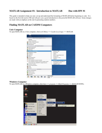
1.15 Graphics15Fig. 1.1 2D plot of asinus10.80.60.40.20 0.2 0.4 0.6 0.8 1 4 3 2 101234Table 1.7 Some graphics commandsTitlexlabelylabelAxis([xmin ,xmax ,ymin ,ymax ])Axis autoAxis squareAxis equalAxis offAxis onTitlex-axis legendy-axis legendSets limits to axisAutomatic limitsSame scale for both axisSame scale for both axisRemoves scaleScales againWe can insert a title, legends, modify axes etc., as shown in table 1.7.By using hold on we can produce several plots in the same figure. We can alsomodify colors of curves or points, as in x 0:.01:2*pi; y1 sin(x); y2 sin(2*x); y3 sin(4*x); plot(x,y1,’--’,x,y2,’:’,x,y3,’ ’)producing the plot of figure 1.2.1.15.2 3D plotsAs for 2D plots, we can produce 3D plots with plot3 using x, y, and z vectors.For examplet .01:.01:20*pi; x cos(t); y sin(t); z t. 3; plot3(x,y,z)produces the plot illustrated in figure 1.3.The next statements produce the graphic illustrated in figure 1.4.
16Fig. 1.2 Colors andmarkers1 Short introduction to MATLAB10.80.60.40.20 0.2 0.4 0.6 0.8 101234567Fig. 1.3 3D plotx 1052.521.510.50110.50.500 0.5 0.5 1 1 [xx,yy] meshgrid(x,x); z exp(-xx. 2-yy. 2); surf(xx,yy,z,gradient(z))1.16 Linear algebraIn our finite element calculations we typically need to solve systems of equations,or obtain the eigenvalues of a matrix. MATLAB has a large number of functions forlinear algebra. Only the most relevant for finite element analysis are here presented.
1.16 Linear algebra17Fig. 1.4 Another 3D plot10.80.60.40.20221100 1 1 2 2Consider a linear system AX B, where a rand(3)a 0.89090.13860.95930.14930.54720.2575 b rand(3,1)b 0.24350.92930.35000.84070.25430.8143The solution vector X can be easily evaluated by using the backslash command, x a\bx 0.78372.9335-1.0246Consider two matrices (for example a stiffness matrix and a mass matrix), forwhich we wish to calculate the generalized eigenproblem. a rand(4)a 0.19660.25110.61600.4733 b .75370.38040.56780.07590.0540
181 Short introduction to MATLABb 0.53080.56880.77920.46940.93400.01190.12990.3371 [v,d] eig(a,b)v 33d 0-0.40440.0394-1.0000000.182200000.7628The MATLAB function eig can be applied to the generalized eigenproblem, producing matrix V, each column containing an eigenvector, and matrix D, containingthe eigenvalues at its diagonal. If the matrices are the stiffness and the mass matrices then the eigenvectors will be the modes of vibration and the eigenvalues willbe the square roots of the natural frequencies of the system.
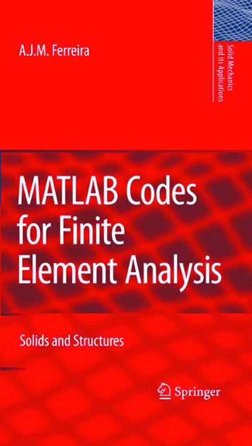
Chapter 2Discrete systems2.1 IntroductionThe finite element method is nowadays the most used computational tool, in science and engineering applications. The finite element method had its origin around1950, with reference works of Courant [1], Argyris [2] and Clough [3].Many finite element books are available, such as the books by Reddy [4], Onate[5], Zienkiewicz [6], Hughes [7], Hinton [8], just to name a few. Some recent booksdeal with the finite element analysis with MATLAB codes [9,10]. The programmingapproach in these books is quite different from the one presented in this book.In this chapter some basic concepts are illustrated by solving discrete systemsbuilt from springs and bars.2.2 Springs and barsConsider a bar (or spring) element with two nodes, two degrees of freedom, cor(e)(e)responding to two axial displacements u1 , u2 ,1 as illustrated in figure 2.1. Wesuppose an element of length L, constant cross-section with area A, and modulusof elasticity E. The element supports axial forces only.The deformation in the bar is obtained as u2 u 1L(e)(2.1)while the stress in the bar is given by the Hooke’s law asσ E (e) E (e)1u2 u1L(e)(2.2)The superscript(e) refers to a generic finite element.A.J.M. Ferreira, MATLAB Codes for Finite Element Analysis:Solids and Structures, Solid Mechanics and Its Applications 157,c Springer Science Business Media B.V. 2009 19
202 Discrete systems(e)u1(e)(e)12 u2(e)(e)R1R2L(e)Fig. 2.1 Spring or bar finite element with two nodesThe axial resultant force is obtained by integration of stresses across the thicknessdirection asu2 u1(2.3)N A(e) σ (EA)(e)L(e)(e)(e)Taking into account the static equilibrium of the axial forces R1 and R2 , as (e)(e)R2 R1 N EAL (e)(e)(e)(u2 u1 )we can write the equations in the form (taking k (e) EAL ) (e)(e)1 1u1R1(e)(e)q k K(e) a(e)(e)(e) 1 1R2u2(2.4)(2.5)where K(e) is the stiffness matrix of the bar (spring) element, a(e) is the displacement vector, and q(e) represents the vector of nodal forces. If the elementundergoes the action of distributed forces, it is necessary to transform those forcesinto nodal forces, by (e) (bl)(e) 11 1u1(e)(e) K(e) a(e) f (e) (2.6)q k(e)1 1 12u2with f (e) being the vector of nodal forces equivalent to distributed forces b.2.3 Equilibrium at nodesIn (2.6) we show the equilibrium relation for one element, but we also need toobt
the remainder of the book. A deeper study of MATLAB can be obtained from many MATLAB books and the very useful help of MATLAB. 1.2 Matrices Matrices are the fundamental object of MATLAB and are particularly important in this book. Matrices can be created in MATLAB in many ways, the simplest one o