Transcription
TECHNICAL BRIEFExamples of Programmingin MATLAB
The MATLAB EnvironmentMATLAB integrates mathematical computing, visualization, and a powerful language to provide a flexible environmentfor technical computing. The open architecture makes it easy to use MATLAB and its companion products to exploredata, create algorithms, and create custom tools that provide early insights and competitive advantages.TABLE OF CONTENTS2Introduction to the MATLAB Language ofTechnical Computing3Comparing MATLAB to C: Three ProgrammingApproaches to Quadratic Minimization4Application Development in MATLAB: Tuning M-fileswith the MATLAB Performance Profiler9TECHNICAL BRIEF
Introduction to the MATLAB Language of Technical ComputingThe MATLAB language is particularly well-suited to designing predictive mathematical models and developingapplication-specific algorithms.It provides easy access to a range of both elementary and advanced algorithms for numeric computing. These algorithmsinclude operations for linear algebra, matrix manipulation, differential equation solving, basic statistics, linear datafitting, data reduction, and Fourier analysis. MATLAB Toolboxes are add-ons that extend MATLAB with specializedfunctions and easy-to-use graphical user interfaces. Toolboxes are accessible directly from the MATLAB interactiveprogramming environment.MATLAB employs the same language for both interactive computing and structured programming. The intuitive mathnotation and syntax allow you to express technical ideas just as you would write them mathematically. This familiarstyle and flexibility make exploration and development with MATLAB very efficient.The built-in math algorithms, optimized for matrix and vector calculations, allow you to increase efficiency in two areas:more productive programming and optimized code performance. The resulting time savings give you fast developmentcycles as well as execution speeds from within the MATLAB environment that are comparable to compiled code.The two examples on the following pages illustrate MATLAB in use:1) The first example compares MATLAB to C using three approaches to a quadratic minimization problem.2) The second example describes one user’s application of the M-file performance profiler to increaseM-file code performance.These examples demonstrate how MATLAB’s straightforward syntax and built-in math algorithms enable developmentof programs that are shorter, easier to read and maintain, and quicker to develop. The embedded code samples, developedby MATLAB users in the MATLAB language, illustrate how MATLAB application specific toolbox functionality can beeasily accessed from the MATLAB language.Examples of Programming in M ATLAB3
COMPARING MATLAB TO C:THREE PROGRAMMING APPROACHES TO QUADRATIC MINIMIZATIONIntroductionQuadratic minimization is a specific form of nonlinear minimization. When a problem has a quadratic objective functioninstead of a general nonlinear function (such as in standard linear least squares), we can find a minimizer more accuratelyand efficiently by taking advantage of the quadratic form. This is particularly true when the quadratic problem is convex.Some examples of these types of applications include: Solving contact and friction problems in rigid body mechanics, typical of the kind encountered in aerospace applications Solving journal bearing lubrication problems, useful for machine design and maintenance planning Computing flow through a porous medium, a common application in chemistry Selecting the best portfolio of financial investmentsIn this example we will use quadratic programming to solve a minimization problem. This example demonstrates the useof MATLAB to simplify an optimization task and compares that solution to the alternative C programming approach. Thethree following code examples compare three approaches to the minimization problem: MATLAB The MATLAB Optimization Toolbox C code including calls to LAPACK, the library that makes up much of the mathematical core of MATLABProblem StatementMinimize a quadratic equation such asy 2x 12 20x 22 6x1x2 5x1with the constraint thatx1 – x2 –2SolutionExpress the original equation in standard quadratic form. First, transform the original equation into matrix notation x1 Ty * x24x16* 6 40 *x25 T x1 0 * x2such that 1 x1–1 * x –22Second, substitute variable names for the vectors and matrices 465H 6 40 , f 04 x1, A 1 –1 , b –2 and x x2TECHNICAL BRIEF
Third, rewrite the quadratic equation asy 5 * x T * H * x 1f T* xand the constraint equation asA * x b.The surface is the graphical representation of the quadratic functionthat we are minimizing, subject tothe constraint that x1 and x2 lieon the line x1 – x2 –2 (represented by the blue line in the smallgraphic and the dashed black linein the large graphic). This blue linerepresents the null space of theequality constraint. The black curverepresents the values on the quadratic surface where the equalityconstraint is satisfied. We startfrom a point on the surface (theupper cyan circle) and the quadratic minimization takes us to thesolution (the lower cyan circle).The quadratic form of the equation is easier to understand and to solve using MATLAB’s matrix-oriented computing language.Having transformed the original equation, we’re ready to compare the three programming approaches.Example 1: Quadratic Minimization with MATLAB M codeMATLAB’s matrix manipulation and equation solving capabilities make it particularly well-suited to quadratic programming problems. The constraint stated above is that A * x b. In the example below we specify four values of b for which xmust be solved, corresponding to the four rows of matrix A. In general, the data is determined by the known parametersof the problem. For example, to solve a financial optimization problem, such as portfolio optimization, the data would bedetermined by the expected return of the investments in the portfolio and the covariance of the returns. Then we wouldsolve for the optimal weighting of the investments by minimizing the variance in the portfolio while requiring the sum ofthe weights to be unity.In this example, we use synthetic data for H, f, A, and b. Once we set up these variables, the next step is to solve for theunknown, x. The code below roughly follows these steps:1) Find a point in six-dimensional space that satisfies the equality constraints A * x b (6 is the number of columns in Hand in A).Examples of Programming in M ATLAB5
2) Project the problem into the null space of A, that is, project into a subspace where movement in that subspace will notviolate these constraints.3) Minimize in this subspace. As our objective is a convex quadratic, we find the minimizer by stepping to the point atwhich the gradient is equal to 0, one Newton step.4) Calculate the final answer by projecting the step to the minimizer and back into the original full space.The following MATLAB M code, solves the type of minimization problem described above. This example has 6 variablesand 4 constraints. The following assignment statements assign the data to the variables H (matrix), f (vector), A (matrix),and b (vector), respectively. The dimensionality of the problem, in this case 6, is specified implicitly by the number ofcolumns in H and A. Note that in MATLAB code, lines preceded by “%” are comments.%% minimize% x1/2*x'*H*x f'*x% 6 dimensional problem with%H [36 17 19 12 8 15; 17 3312 11 13 18 6 11; 8 7 8 6f [ 20 15 21 18 29 24 ]';A [ 7 1 8 3 3 3; 5 0 5 1 5b [ 84 62 65 1 ]';Z null(A);x A\b;g H*x f;Zg Z'*g;ZHZ Z'*H*Z;t -ZHZ \ Zg;xsol x Z*t;%%%%%%%%%such that A*x b4 constraints:18 11 7 14; 19 18 43 13 8 16;9 8; 15 14 16 11 8 29];8; 2 6 7 1 1 8; 1 0 0 0 0 0 ];Find the null space of constraint matrix ADetermine an x satisfying the equality constraints A*x bCompute the gradient (first derivative vector) of the quadraticequation at xFind the projected gradientCompute the projected Hessian matrix (second derivative matrix)Solve for the projected Newton stepProject the step back into the full space and add to x to findthe solution xsolExample 2: Quadratic Minimization with the Optimization ToolboxWe can also solve the problem in Example 1 using the MATLAB Optimization Toolbox. It turns out that quadprog,the quadratic programming function in the Optimization Toolbox, can solve the entire problem described above. Thefollowing code could be typed in at the MATLAB command line or saved in a “script” file and run from MATLAB. Oncethe four MATLAB variable assignments are executed (the same ones as in Example 1), and some options are set, the call toquadprog is all that is required to solve the above problem.H [36 17 19 12 8 15; 17 33 18 11 7 14; 19 18 43 13 8 16;12 11 13 18 6 11; 8 7 8 6 9 8; 15 14 16 11 8 29];f [ 20 15 21 18 29 24 ]';A [ 7 1 8 3 3 3; 5 0 5 1 5 8; 2 6 7 1 1 8; 1 0 0 0 0 0 ];b [ 84 62 65 1 ]';options optimset (‘largescale’,’off’);xsol L BRIEF
Example 3: Quadratic Minimization in C and LAPACKWhat would the equivalent C code implementation look like for the same problem?Assume that you have the C code version of the LAPACK linear algebra subroutine library and the BLAS subroutinelibrary at your disposal. The following code uses the LAPACK subroutines dgesv, dgelsx, dgesvd, and the BLASroutines daxpy, dgemm, and dgemv. (Without these functions, you would need to write the numerical linear algebraroutines in C directly). Here is the resulting C program, totaling 70 lines:#include stdio.h #include math.h #include ntegerm 4;n 6;nrhs 1;max1 max(min(m,n) 3*n,2*min(m,n) nrhs);max2 max(3*min(m,n) max(m,n),5*min(m,n)-4);lwork max(max1,max2);/* for dgelsx *//* for dgesvd *//* for both *//* Problemdouble A[]double b[]double H[]definition arrays (column order) */ {7,5,2,1, 1,0,6,0, 8,5,7,0, 3,1,1,0, 3,5,1,0, 3,8,8,0}; {84,62,65,1}; {36,17,19,12,8,15, 17,33,18,11,7,14, 19,18,43,13,8,16,12,11,13,18,6,11, 8,7,8,6,9,8, 15,14,16,11,8,29};double f[] {20,15,21,18,29,24};double *QR, *x, *work, *g, *s, *U, *VT, *Z, *ZH, *ZHZ, *Zg;double *p1, *p2, rcond, one 1.0, zero 0.0, minusone -1.0;integer *jpvt, *ipiv, rankA, nullA, info, inc 1, i, j;char jobu 'N', jobvt 'A', transn 'N', transt 'T';/* Allocate contiguous memory for work arrays */QR malloc( m*n*sizeof(double) );x malloc( n*sizeof(double) );work malloc( lwork*sizeof(double) );g malloc( n*sizeof(double) );s malloc( m*sizeof(double) );U NULL;VT malloc( n*n*sizeof(double) );Z malloc( n*n*sizeof(double) );ZH malloc( n*n*sizeof(double) );ZHZ malloc( n*n*sizeof(double) );Zg malloc( n*sizeof(double) );jpvt malloc( n*sizeof(int) );ipiv malloc( n*sizeof(int) );/* QR A: since it will be overwritten by dgelsx */for (i 0, p1 QR, p2 A; i m*n; i )*p1 *p2 ;/* x b: since it will be overwritten by dgelsx */for (i 0, p1 x, p2 b; i m; i )Examples of Programming in M ATLAB7
*p1 *p2 ;/* x A \ b: solve min b - A*x for x, using a QR factorization of A */dgelsx (&m, &n, &nrhs, QR, &m, x, &n, jpvt, &rcond, &rankA, work, &info);/* g H * x */dgemv (&transn, &n, &n, &one, H, &n, x, &inc, &zero, g, &inc);/* g g f */daxpy (&n, &one, f, &inc, g, &inc);/* Z null(A) *//* [U,S,V] svd(A) */dgesvd (&jobu, &jobvt, &m, &n, A, &m,s, U, &m, VT, &n, work, &lwork, &info);/* dimension of null space of A */nullA max(m,n) - rankA;/* Z last nullA columns of V (last nullA rows of VT) */for (j 0; j nullA; j )for (i 0; i n; i )Z[i j*n] VT[(i 1)*n-nullA j];/* ZHZ Z' * H * Z */dgemm (&transt, &transn, &nullA, &n, &n,&one, Z, &n, H, &n, &zero, ZH, &n);dgemm (&transn, &transn, &nullA, &nullA, &n,&one, ZH, &n, Z, &n, &zero, ZHZ, &n);/* Zg Z' * g */dgemv (&transt, &n, &nullA, &one, Z, &n, g, &inc, &zero, Zg, &inc);/* Zg ZHZ \ Zg */dgesv (&nullA, &nrhs, ZHZ, &n, ipiv, Zg, &n, &info);/* g - Z * Zg; */dgemv (&transn, &n, &nullA, &minusone, Z, &n, Zg, &inc, &zero, g, &inc);/* x x g */daxpy (&n, &one, g, &inc, x, &inc);printf(" \n");for (i 0; i n; i ) {printf("%f\n",x[i]);}printf(" \n");}As you can see, except for the calls to the LAPACK routines and the comments, the remaining C code consists almostexclusively of variable declarations and memory allocation via calls to malloc.8TECHNICAL BRIEF
Comparing the Three Programing ApproachesClearly, it is possible to solve the minimization problem using MATLAB, the Optimization Toolbox, or standard C. Allthree approaches run and produce correct answers. The primary differences between them are code length and overallcomplexity.The following table summarizes the number of lines of code required for each solutionMATLAB code example:11 lines (including 4 lines of data definitions)Optimization Toolbox example:6 lines (including 4 lines of data definitions)C code example:70 lines (including 14 lines of declarations and13 lines of memory allocation)Both the MATLAB and Optimization Toolbox examples are fairly short and straightforward to follow. MATLAB accomplishes the task in 6 lines or 11 lines, depending on the approach. It requires 70 lines of C code to do what MATLAB couldhandle in 1/10 of that. In this case, the LAPACK industry-tested library contained the required routines to perform thenecessary foundation numeric computations. Corresponding routines to those available in MATLAB and the complementary application specific toolboxes may not always be so reliable and easily accessible when solving other types of problems.The C code version is much more difficult to read and understand than the corresponding MATLAB code that performsessentially the same steps. In addition, C, like many high-level languages, requires memory management, variable initializations, and variable declarations. These additional steps not only take up space, but require additional programming,debugging, and testing time. By comparison, MATLAB handles these overhead tasks behind the scenes, thereby savingtime and allowing you to create more readable and maintainable code.APPLICATION DEVELOPMENT IN MATLAB:TUNING M-FILES WITH THE MATLAB PERFORMANCE PROFILERMany users have found MATLAB to be a very productive environment for experimenting with and comparing differentapproaches to application development. The three examples in the preceding section illustrate how MATLAB can helpyou shorten your development cycles and thereby save you time.A number of MATLAB programming tools make it possible to not only develop solutions, but also to refine your prototypes and iterate on your designs. These tools include the MATLAB color-coded visual editor/debugger, the online hotlinked reference documentation, and the M-file performance profiler.The performance profiler monitors the computing time spent on each line of code for a particular MATLAB M-file function. This information can provide you with insight into which operations are the most time-intensive, perhaps givingimplicit clues about which computing tasks to tune or even replace with different, faster alternatives.In the following example we apply the M-file performance profiler to a digital image processing application involvingobject measurement.A number of image processing applications rely on the ability to measure and compare the characteristics of similarobjects. This type of object measurement is useful in applications such as: Medical research, for example the study of cancer cells Quality control applications involving inspection sampling and process monitoring Analysis of satellite imagery, such as the object enhancement and measurement of rocks in photographs during theSojourner Mars missionExamples of Programming in M ATLAB9
In the following profiler summary report, the first few lines list the total execution time (2.18 seconds) and the lines thatconsumed the most computing time, in descending order of time. Three numbers precede the code on each of the individual code lines: the computing time in seconds, the percentage of the total time, and the number of lines of code in theoriginal M-file routine.The complete function, imfeature.m, is 220 lines long. In the interest of space, the entire function is not included here butthe relevant portions are shown. After profiling an execution of imfeature.m, the profiler generates this summary report:profile reportTotal time in "h:\ipt2.1\imfeature.m": 2.18 seconds79% of the total time was spent on lines:[25 219 20 40 218 90 3 220 214 209]2:0.05s, 2%3: numObjs round(max(L(:)));4: if (numObjs 0)0.24s, 11%19: elementValues L(idx);20: S sparse(idx, elementValues, ones(size(elementValues)));21: objRowCoordinates cells(1,numObjs);24: for k 1:numObjs0.52s, 24%25:[objRowCoordinates{k},objColCoordinates{k}] ind2sub(sizeL . . .26: end0.14s, 6%39:stats(k).EulerNumber eulerNumber;40:stats(k).Centroid [mean(r) mean(c)];41: end0.07s, 3%89: lut aglut;90: markers applylut(BW, lut);91: numQ1 length(find(markers 1));0.04s, 2%208:209: minR min(r);210: maxR max(r);0.04s, 2%213: r r - minR 2;214: c c - minC 2;215: M maxR - minR 1;0.09s, 4%0.49s, 22%0.04s, 2%217:218:219:220:BW uint8(0);BW repmat(BW, M 2, N 2);idx sub2ind([M 2, N 2], r, c);BW(idx) 1;The report shows that imfeature is spending 22% of the time in calls to sub2ind (on line 219). Looking at thesubind code, we can see that much of sub2ind handles general cases that aren’t relevant to this particular useof sub2ind. As a result, we inserted the useful lines of code from sub2ind directly in the imfeature function,eliminating the calls to the sub2ind function.10TECHNICAL BRIEF
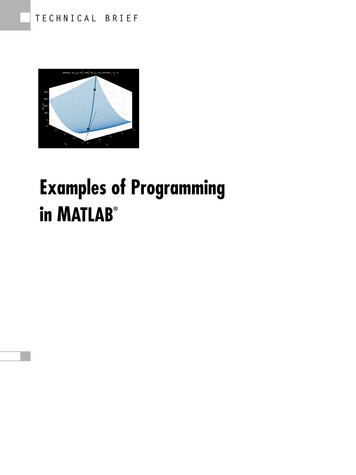
After making the code changes, we ran the profiler on the modified imfeature.profile reportTotal time in "h:\ipt2.1\imfeature.m": 1.77 seconds77% of the total time was spent on lines:[25 20 40 218 90 93 3 210 221 219]2:0.05s, 3%3: numObjs round(max(L(:)));4: if (numObjs 0)0.23s, 13%19: elementValues L(idx);20: S sparse(idx, elementValues, ones(size(elementValues)));21: objRowCoordinates cells(1,numObjs);0.53s, 30%24: for k s{k}] ind2sub(sizeL . . .)26: end0.22s, 12%39:stats(k).EulerNumber eulerNumber;40:stats(k).Centroid [mean(r) mean(c)];41: end0.07s, 4%89: lut aglut;90: markers applylut(BW, lut);91: numQ1 length(find(markers 1));92: numQ2 length(find(markers 2));0.05s, 3%93: numQ3 length(find(markers 3));94: numQ4 length(find(markers 4));0.04s, 2%0.11s, 6%0.03s, 2%0.03s, 2%209: minR min(r);210: maxR max(r);211: minC min(c);217:218:219:220:221:222:BW uint8(0);BW repmat(BW, M 2, N 2);idx (M 2)*(c-1) r;%%% idx sub2ind([M 2, N 2], r, c);BW(idx) 1;We see above that the call to sub2ind is commented out (line 220) and replaced with an inline assignment statementon line 219.This second profile report shows that imfeature now takes 1.77 seconds, a savings of 19%. Specifically, the inlinecomputation takes 0.03 seconds, compared with 0.44 seconds previously.Not bad for a single, quick change but we could certainly pursue further optimizations such as investigating whetherthe code on line 25, now taking up 30% of the total execution time, could be further tuned. This example is just oneillustration of the savings possible with the various programming tools available in the MATLAB environment. 2001 by The MathWorks, Inc. MATLAB, Simulink, Stateflow, Handle Graphics, and Real-Time Workshop are registered trademarks, and Target Language Compiler is a trademark of The MathWorks, Inc. Other product or brand names are trademarks or registered trademarks of theirrespective holders.
For demos, application examples,tutorials, user stories, and pricing: Visit www.mathworks.com Contact The MathWorks directlyUS & Canada 508-647-7000BeneluxFranceGermanySpainSwitzerlandUK 31 (0)182 53 76 44 33 (0)1 41 14 67 14 49 (0)89 995901 0 34 93 362 13 00 41 (0)31 954 20 20 44 (0)1223 423 200Visit www.mathworks.com to obtaincontact information for authorizedMathWorks representatives in countriesthroughout Asia Pacific, Latin America,the Middle East, Africa, and the restof Europe.The MathWorks9514v02 08/01
Comparing MATLAB to C: Three Programming Approaches to Quadratic Minimization Application Development in MATLAB: Tuning M-files with the MATLAB Performance Profiler 3 4 9. Introduction to the MATLAB Language of Technical Computing The MATLAB language is particularly well-suited t