WIXLIB

Accepted to the 3rd IFAC Conference on Advances in Proportional-Integral-Derivative Control,Ghent, Belgium, May 9-11, 2018THj (XBaugj N )R 1 (BaugP NT )j 1T (P Baugj N )R (Baugj X N T )TX N T ). (XBaugj N )R 1 (Baugj(13)Proof 1. Let us choose the Lyapunov function as:V (t) x̃(t)T P x̃(t),(14)The first derivative of the Lyapunov function (14) is then: T P x̃(t) x̃(t)T P x̃(t) V̇ (ξ(t)) x̃(t) (15) x̃(t)T Ac (ξ(t))T P P Ac (ξ(t)) x̃(t),whereAc (ξ(t)) Aaug (ξ(t)) Baug (ξ(t))F Caug (ξ(t)). (16)By substituting the control law (7) to the cost function (1)we can obtain:Z x̃(t)T J(ξ(t))x̃(t)dtJ (17)0whereJ(ξ(t)) Q Caug (ξ(t))T F T RF Caug (ξ(t))(18) N F Caug (ξ(t)) Caug (ξ(t))T F T N T .By summarizing the equations (15) and (18) the BellmanLyapunov inequality can be obtained in the form:M (ξ(t)) V̇ (ξ(t)) J(ξ(t)) 0,(19)Furthermore, if P is positive definite then the BellmanLyapunov inequality (19) can be rewritten to this form:V̇ (ξ(t)) J(ξ(t)) 0 V̇ (ξ(t)) J(ξ(t)) 0 (20)Integrating both sides form 0 to one can obtain:J V (0) V ( ) x̃(0)T P x̃(0).(21)It follows that by minimizing trace(P ) and by satisfyingM (ξ(t)) 0 as well as P 0, the closed-loop systemwill be quadratically stable with guaranteed cost definedby (21). In order to obtain LMI conditions, the matrixM (ξ(t)) can be rewritten to:M (ξ(t)) Ac (ξ(t))T P P Ac (ξ(t) Q Caug (ξ(t))T F T RF Caug (ξ(t))T(22)TT N F Caug (ξ(t)) Caug (ξ(t)) F N .Let us define: G(ξ(t)) F Caug (ξ(t)) R 1 Baug (ξ(t))T P N T (23)Substituting (23) to (22) and applying the Schur complement we can obtain: M11 (ξ(t)), G(ξ(t))TM (ξ(t)) ,(24)G(ξ(t)), R 1whereM11 (ξ(t)) A(ξ(t))T P P A(ξ(t)) Q H(ξ(t)), (25)H(ξ(t)) (P B(ξ(t)) N )R 1 (B(ξ(t))T P N T ). (26)Since M (ξ(t)) is convex in the uncertain parameter ξ,therefore M (ξ(t)) will be negative semi-definite if and onlyif it is negative semi-definite at the corners of ξ. Hence,semi-definiteness splits to p inequalities (9).Remark 4. For the first iteration X 1 is a freely chosenpositive definite matrix. It can be set by the designer or canbe calculated/approximated by a standard LQR designusing the nominal system.Remark 5. The weighting matrices Q, R and N are alsoaugmented since the state and control input vectors areaugmented as well.3. FUNCTION DESCRIPTIONThe following command (in Matlab/Octave):[F,P,E] oflqr(sys,Q,R,N,ct,Opt) calculates the(sub)optimal robust structurable output-feedback gainmatrix F such that, for a continuous-time polytopic statespace model sys, the output-feedback law defined withct (control type: P, PI, PID, PD, D or DOF, DOFI,DOFID, DOFD) guarantees the robust closed-loop stability (quadratic stability) and minimizes the cost function(1), subject to the system dynamics:ẋ(t) Aj x(t) Bj u(t), j 1, . . . , p(28)y(t) Cj x(t); yi (t) Cij x(t); yd (t) Cdj x(t),where x(t), u(t) and y(t) are state, control input and measurable output vectors, respectively. Furthermore, yi (t)and yd (t) are measurable output vectors for the integraland derivative parts of the controller.INPUTSREQUIRED:SYS - state-space LTI systems (in convex polytopicform). array of ss models: sys(:,:,1:p), (Matlab). cels of ss objects: sys{1:p}, (Matlab, Octave). single ss object: sys, (Matlab, Octave)Q- weighting matrix related to states (Q 0 ifN 0)R- positive definite weighting matrix (R 0)N- If N 6 0 then Q N R 1 N T 0 (use eig tocheck)ct. ct ’p’: Proportional (P) controlleru(t) Kp y(t),(29)F [Kp ].(30). ct ’pi’: Proportional-Integral (PI) controllerZ tu(t) Kp y(t) Kiyi (t)dt,(31)0(27)F [Kp , Ki ].(32).ct ’pid’:Proportional-Integral-Derivative(PID) controllerZ tu(t) Kp y(t) Kiyi (t)dt Kd ydf (t), (33) (XBaug (ξ(t)) N )R 1 (Baug (ξ(t))T X N T ),hence, we get an iterative procedure, where in each iteration holds X i P i 1 (i - actual iteration step). Theiteration ends if trace(Pi ) trace(Pi 1 ) , where canbe set by the designer.F [Kp , Ki , Kd ],(34)where ydf is the vector of filtered derivatives,using derivative filter (5) (default N f 100). ct ’pd’: Proportional-Derivative (PD) controllerWe can linearize the nonlinear part in (26) as:lin(H(ξ(t))) (XBaug (ξ(t)) N )R 1 (Baug (ξ(t))T P N T ) (P Baug (ξ(t)) N )R 1 (Baug (ξ(t))T X N T )0

Accepted to the 3rd IFAC Conference on Advances in Proportional-Integral-Derivative Control,Ghent, Belgium, May 9-11, 2018u(t) Kp y(t) Kd ydf (t),(35)F [Kp , Kd ],(36)where ydf is the vector of filtered derivatives,using derivative filter (5) (default N f 100). ct ’d’: Derivative (D) controlleru(t) Kd ydf (t),(37)F [Kd ],(38)where ydf is the vector of filtered derivatives,using derivative filter (5) (default N f 100). ct ’dof’: Dynamic output-feedback with order nc (default nc 2)ẋc (t) Ac xc (t) Bc y(t),(39)u(t) Cc xc (t) Kp y(t), Kp , CcF .(40)Bc , Ac. ct ’dofi’: Dynamic output-feedback withintegral part and order nc (default nc 2)Z tyi (t)dtẋc (t) Ac xc (t) Bc1 y(t) Bc20(41)Z tu(t) Cc xc (t) KP y(t) Kiyi (t)dt,0 Kp , Cc , KiF .(42)Bc2 , Ac , Bc2. ct ’dofd’: Dynamic output-feedbackfiltered derivative part; order nc (default ncẋc (t) Ac xc (t) Bc1 y(t) Bc3 ydf (t),u(t) Cc xc (t) KP y(t) Kd ydf (t), Kp , Cc , KdF .Bc2 , Ac , Bc3with 2)(43)(44)where ydf is the vector of filtered derivatives,using derivative filter (5) (default N f 100). ct ’dofid’: Dynamic output-feedback withintegral and filtered derivative part; order nc(default nc 2)ẋc (t) Ac xc (t) Bc1 y(t)Z t Bc2yi (t)dt Bc3 ydf (t),0(45)u(t) Cc xc (t) KP y(t)Z t Kiyi (t)dt Kd ydf (t),0 F Kp , Cc , Ki , Kd.Bc2 , Ac , Bc2 , Bc3(46)where ydf is the vector of filtered derivatives,using derivative filter (5) (default N f 100).OPTIONAL:Opt - options in structure:. Opt.iter: maximal number of iterations (default: 100). Opt.eps: epsilon for the stopping criteria (default: eps 10 8 ). Opt.epsP: epsilon for the positive definitenesstest P epsP I (default: epsP 2.2204 10 16 ). Opt.X: Initial Lyapunov matrix for the iteration. If X 0 then it is calculated by lqrcommand. (default: X 0). Opt.nc: Order of the dynamic controller. i.e.:nc 3.(default: nc 2). Opt.Nf: Filter constant for the derivative filter.Gf (s) Nf s/(s Nf ). (default Nf 100). Opt.CS: Controller structure matrix - whichdescribes the controller structure. CS has the sizeof F and contains 1 or 0. i.e.: for ct ’p’, andfor m l, to obtain fully decentralized controlCS eye(m,l). (default CS ones(size(F))). Opt.Ci: Output matrix for Integral part. (default Ci C). Opt.Cd: Output matrix for Derivative part.(default Cd C). Opt.settings: Options structure for Yalmip(sdpsettings). The structure is same as forthe sdpsettings: {’name’, value,.}. i.e.:Opt.settings {’solver’,’sdpt3’}.OUTPUTSF - static output-feedback gain matrixP - Lyapunov matrixE - Closed-loop system eigenvaluesOTHER INFOWeighting matrix size (Q,R,N):ct ’p’:Q(n,n), R(m,m), N(n,m)ct ’pi’:Q(n li,n li), R(m,m),N(n li,m)ct ’pid’:Q(n li ld,n 2*li ld),R(m,m), N(n li ld,m)ct ’pd’:Q(n ld,n ld), R(m,m),N(n ld,m)ct ’d’:Q(n ld,n ld), R(m,m),N(n ld,m)ct ’dof’:Q(n nc,n nc), R(m nc,m nc),N(n nc,m nc)ct ’dofi’: Q(n nc li,n nc li),R(m nc,m nc),N(n nc li,m nc)ct ’dofid’: Q(n nc li ld,n nc li ld),R(m nc,m nc),N(n nc li ld,m nc)wheren m l li ld nc -number of states,number of inputs,number of outputs,number of outputs for integral part, (def. li l),number of outputs for deriv. part, (def. ld l),order of the dynamic controller (def. nc 2).REQUIREMENTSMatlab:- Control System Toolbox installed.- YALMIP installed (R2015xxx or newer).- LMI solver installed (sdpt3, sedumi, mosek, .).Octave:- Control package installed and loaded.- YALMIP installed (R2015xxx or newer).- LMI solver installed (sdpt3, sedumi, .).

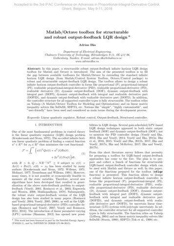
Accepted to the 3rd IFAC Conference on Advances in Proportional-Integral-Derivative Control,Ghent, Belgium, May 9-11, 20184. EXAMPLESIn order to show the viability of the previous proposedmethod, the following examples have been chosen.Example 1. The first example is the Rosenbrock system(Rosenbrock, 1970), which will be used to demonstrateand compare the proposed method with the standard LQRdesign. The transfer function of the system is as follows: 12 , s 3s 1G(s) ,(47)11s 1 , s 1which can be transformed to the form (2) with matrices: 1, 0, 0, 01, 00, 3, 0, 00, 2A 0, 0, 1, 0 , B 1, 0 ,0, 0, 0, 10, 1hihi1, 1, 0, 00, 0C 0, 0, 1, 1 , D 0, 0 .Different controller types were designed using the oflqrfunction. Beside types P, PI, PID, PD, DOF, DOFI,DOFID and DOFD, state-feedbacks like static statefeedback (SSF), dynamic state-feedback (DOF) and theirvariations were also designed (by changig the C matrix).Numerical solution has been carried out by SDPT3 (Tohet al., 1999) solver under OCTAVE 4.0 using YALMIPR20150918 (Löfberg, 2004). The obtained guaranteed cost(J ) for x0 [1, 1, 1, 1], Q In , R Im and N 0.1 ones(n , m ) can be found in Table 1. (n , m denotesthe augmented number of states and inputs for the givencontrol type).Table 1. Controller types & guaranteed costsController typeStandard infinite-horizon LQR:. SSFProposed method:. SSF. SSFI. SSFID. SSFD. DSF (nc 1). DSF (nc 2). DSFI (nc 2). DSFID (nc 2). DSFD (nc 2). Centralized P. Decentralized P. Centralized PI. Decentralized PI. Centralized PID. Decentralized PID. Centralized PD. Decentralized PD. Centralized DOF (nc 1). Centralized DOF (nc 2). Decentralized DOF (nc 2). Centralized DOFI (nc 2). Centralized DOFID (nc 2). Decentralized DOFID (nc 2). Centralized DOFD (nc 2)J Example 2. The second example is the aircraft pitch control problem from the Control Tutorials for Matlab andSimulink (Messner et al., 2017). The state-space model forone of Boeing’s commercial aircraft is given as: "#" # "#α̇ 0.313, 56.7, 0α0.232 q̇ 0.0139, 0.426, 0q 0.0203 δ,(48)0,56.7, 0θ0θ̇y [0, 0, 1][α, q, θ]TFig. 1. Step response for 0.2 radianswhere α is the angle of attack, q is the pitch rate, θ isthe pitch angle and δ is the elevator deflection angle. Thedesign requirements are the following: overshoot less than10%, rise time less than 2 seconds, settling time less than10 seconds, steady-state error less than 2%.Using the LQR-based controller design approaches thecontroller parameter’s tuning is replaced by the tuningof the weighting parameters. This can relevantly reducethe time and complexity of the tuning process, mainlyfor large-scale multi-input multi-output applications. Formore information and tuning approaches the readers arereferred to books (Athans and Falb, 1966; Dorato et al.,2000) and references therein.After a short iterative tuning all the requirements werefulfilled by Q diag([0, 0, 0, 0.6, 28]), R 1 and N [0; 0; 0; 0; 4.5] (step response: Fig. 1) with rise time: 0.954seconds, settling time: 9.5603 seconds, overshoot: 7.496%,steady-state error: 0%. The obtained realizable PID gainsare: Kp 5.1724, Ki 1.7031, Kd 3.0076, with filtercoefficient Nf 100.Example 3. The third example is a simple uncertainMIMO system, which will be used to demonstrate thefreedom in structurability what the oflqr can give. Forexample, different controller types can be designed for eachsubsystem at once. The system with parametric uncertainty is given as:"#h1,2i2,s 1G(s) 10s 1(49)h 3, 4i ,1s 1 ,10s 1which can be transformed to the form (2) with matrices: 0.1, 0, 0, 00.1, 00, 1, 0, 00, 2A1,2,3,4 0, 0, 1, 0 , B1 1, 0 ,0, 0.30, 0, 0, 0.1 0.2, 00.2, 00.1, 00, 20, 20, 2B2 1, 0 , B3 1, 0 , B4 1, 0 0, 0.40, 0.40, 0.3ihih1, 1, 0, 00, 0C1,2,3,4 0, 0, 1, 1 , D1,2,3,4 0, 0 .Assume that we want to design a fully decentralizedcontroller, more precisely a PI controller for the firstsubsystem and a PID for the second subsystem. In orderto do so, let’s define the output matrix for the derivativepart just for the second subsystem: Opt.Cdj Cj(2,:).Finally, let us construct the structure matrix Opt.CS:

Accepted to the 3rd IFAC Conference on Advances in Proportional-Integral-Derivative Control,Ghent, Belgium, May 9-11, 2018y1y2 z1 z2 ydf2i1,0, 1, 0, 0 .CS (50)0, 1, 0, 1, 1Numerical solution has been carried out by SDPT3 (Tohet al., 1999) solver under OCTAVE 4.0 using YALMIPR20150918 (Löfberg, 2004). The obtained PI and PIDgains by weighting matrices Q In li ld , R Im andN 0n li ld m are as follows:PI: Kp 1.6344, Ki 1.0014,PID: Kp 1.2735, Ki 0.5119,(51)Kd 0.0403.u1u2h5. CONCLUSIONA new toolbox for Matlab and Octave is introduced in thispaper. More precisely a function from the toolbox, whichcan be used to design a structurable robust LQR-basedoutput feedback controller for uncertain LTI systems. Thetoolbox will soon be enriched by the discrete version of thepresented oflqr function. Moreover, the future plan is toinclude the author’s all recent results in linear parametervarying (LPV)/ gain-scheduled output-feedback controllerdesign as functions in the presented toolbox. For recentupdates please visit: , M. and Falb, P. (1966). Optimal control. McGrawHill Publishing Company, Ltd, Maidenhead, Berksh,New York. Pp. 879.Dorato, P., Abdallah, C.T., and Cerone, V. (2000). LinearQuadratic Control: An Introduction. Krieger PublishingCompany.Engwerda, J. and Weeren, A. (2008). A result on outputfeedback linear quadratic control. Automatica, 44(1),265–271.Ilka, A. and McKelvey, T. (2017). Robust discrete-timegain-scheduled guaranteed cost PSD controller design.In 2017 21st Int. Conference on Process Control, 54–59.Ilka, A. and Veselý, V. (2017a). Robust LPV-basedinfinite horizon LQR design. In 2017 21st InternationalConference on Process Control (PC), 86–91.Ilka, A., Ottinger, I., Ludwig, T., Tárnı́k, M., Veselý, V.,Miklovicová, E., and Murgaš, J. (2015). Robust Controller Design for T1DM Individualized Model: GainScheduling Approach. International Review of Automatic Control (IREACO), 8(2), 155–162.Ilka, A. and Veselý, V. (2014). Gain-Scheduled ControllerDesign: Variable Weighting Approach. Journal of Electrical Engineering, 65(2), 116–120.Ilka, A. and Veselý, V. (2017b). Robust guaranteedcost output-feedback gain-scheduled controller design.IFAC-PapersOnLine, 50(1), 11355 – 11360. 20th IFACWorld Congress.Ilka, A., Veselý, V., and McKelvey, T. (2016). RobustGain-Scheduled PSD Controller Design from Educational Perspective. In Preprints of the 11th IFAC Symposium on Advances in Control Education, 354–359.Bratislava, Slovakia.Kwakernaak, H. and Sivan, R. (1972). Linear optimalcontrol systems. Wiley-Interscience.Löfberg, J. (2004). YALMIP : A Toolbox for Modelingand Optimization in MATLAB. In Proceedings of theCACSD Conference. Taipei, Taiwan.Messner, B., Tilbury, D., and JD, T. (2017). Controltutorials for matlab and simulink. Technical report,Creative Commons Attribution.Molinari, B. (1977). The time-invariant linear-quadraticoptimal control problem. Automatica, 13(4), 347 – 357.Mukhopadhyay, S. (1978). P.I.D. equivalent of optimalregulatror. Electronics Letters, 14(25), 821–822.Rosenbrock, H. (1970). State-Space and MultivariableTheory. Nelson, London, U.K.Rosinová, D. and Veselý, V. (2004). Robust static outputfeedback for discrete-time systems - LMI approach.Periodica Polytechnica Ser. El. Eng., 48(3-4), 151–163.Rosinová, D. and Veselý, V. (2007). Robust PID decentralized controller design using LMI. Int. Journal ofComputers, Communications & Control, 2(2), 195–204.Rosinová, D., Veselý, V., and Kučera, V. (2003). A necessary and sufficient condition for static output feedbackstabilizability of linear discrete-time systems. Kybernetika, 39(4), 447–459.Shamma, J.S. (2012). Control of Linear Parameter Varying Systems with Applications, chapter An overview ofLPV systems, 3–26. Springer.Sturm, J. (1999). Using SeDuMi 1.02, a MATLAB toolboxfor optimization over symmetric cones. OptimizationMethods and Software, 11–12, 625–653.Toh, K.C., Todd, M., and Tütüncü, R.H. (1999). SDPT3 –a MATLAB software package for semidefinite programming. Optimization methods and software, 11, 545–581.Trentelman, H.L. and Willems, J.C. (1991). The Dissipation Inequality and the Algebraic Riccati Equation, 197–242. Springer Berlin Heidelberg, Berlin, Heidelberg.Veselý, V. (2001). Static output feedback controller design.Kybernetica, 37(2), 205–221.Veselý, V. (2005). Static output feedback robust controllerdesign via LMI approach. Journal of Electrical Engineering, 56(1-2), 3–8.Veselý, V. (2006). Robust controller design for linearpolytopic systems. Kybernetika, 42(1), 95–110.Veselý, V. and Ilka, A. (2013). Gain-scheduled PID controller design. Jour. of Process Cont., 23(8), 1141–1148.Veselý, V. and Ilka, A. (2015a). Design of robust gainscheduled PI controllers. Journal of the Franklin Institute, 352(4), 1476 – 1494.Veselý, V. and Ilka, A. (2015b). Unified Robust GainScheduled and Switched Controller Design for LinearContinuous-Time Systems. International Review ofAutomatic Control (IREACO), 8(3), 251–259.Veselý, V. and Ilka, A. (2017). Generalized robust gainscheduled PID controller design for affine LPV systemswith polytopic uncertainty. Systems & Control Letters,105(2017), 6–13.Veselý, V. and Rosinová, D. (2011). Robust PSD Controller Design. In M. Fikar and M. Kvasnica (eds.), Proceedings of the 18th International Conference on ProcessControl, 565570. Tatranská Lomnica, Slovakia.Veselý, V. and Rosinová, D. (2013). Robust PID-PSDController Design: BMI Approach. Asian Journal ofControl, 15(2), 469–478.Willems, J. (1971). Least squares stationary optimal control and the algebraic riccati equation. IEEE Transactions on Automatic Control, 16(6), 621–634.Zhou, K., Doyle, C.J., and Glover, K. (1996). Robust andoptimal control. Prentice-Hall Inc., U.S. River, USA.

toolbox for Matlab and Octave is introduced. The aim of the presented toolbox is to ll the gap between available toolboxes for Matlab/Octave by extending the standard in nite horizon LQR design (from Matlab/Control System Toolbox, Octave/Control package) to robust and structurable output-feedback LQR design. The toolbox allows to design a robust