Transcription
Chapter 8n-dimensional Fourier Transform8.1Space, the Final FrontierTo quote Ron Bracewell from p. 119 of his book Two-Dimensional Imaging, “In two dimensions phenomenaare richer than in one dimension.” True enough, working in two dimensions offers many new and richpossibilities. Contemporary applications of the Fourier transform are just as likely to come from problems intwo, three, and even higher dimensions as they are in one — imaging is one obvious and important example.To capitalize on the work we’ve already done, however, as well as to highlight differences between the onedimensional case and higher dimensions, we want to mimic the one-dimensional setting and argumentsas much as possible. It is a measure of the naturalness of the fundamental concepts that the extensionto higher dimensions of the basic ideas and the mathematical definitions that we’ve used so far proceedsalmost automatically. However much we’ll be able to do in class and in these notes, you should be able toread more on your own with some assurance that you won’t be reading anything too much different fromwhat you’ve already read.Notation The higher dimensional case looks most like the one-dimensional case when we use vectornotation. For the sheer thrill of it, I’ll give many of the definitions in n dimensions, but to raise the comfortlevel we’ll usually look at the special case of two dimensions in more detail; two and three dimensions arewhere most of our examples will come from.We’ll write a point in Rn as an n-tuple, sayx (x1 , x2 , . . . , xn ) .Note that we’re going back to the usual indexing from 1 to n. (And no more periodic extensions of then-tuples either!) We’ll be taking Fourier transforms and may want to assign a physical meaning to ourvariables, so we often think of the xi ’s as coordinates in space, with the dimension of length, and x asthe “spatial variable”. We’ll then also need an n-tuple of “frequencies”, and without saying yet what“frequency” means, we’ll (typically) writeξ (ξ1 , ξ2 , . . . , ξn )for those variables “dual to x”. Recall that the dot product of vectors in Rn is given byx · ξ x1 ξ1 x2 ξ2 · · · xn ξn .The geometry of Rn is governed by the dot product, and using it will greatly help our understanding aswell as streamline our notation.
3368.1.1Chapter 8 n-dimensional Fourier TransformThe Fourier transformWe started this course with Fourier series and periodic phenomena and went on from there to define theFourier transform. There’s a place for Fourier series in higher dimensions, but, carrying all our hard wonexperience with us, we’ll proceed directly to the higher dimensional Fourier transform. I’ll save Fourierseries for a later section that includes a really interesting application to random walks.How shall we define the Fourier transform? We consider real- or complex-valued functions f defined onRn , and write f (x) or f (x1 , . . . , xn ), whichever is more convenient in context. The Fourier transform off (x) is the function Ff (ξ), or fˆ(ξ), defined byZe 2πix·ξ f (x) dx .Ff (ξ) RnThe inverse Fourier transform of a function g(ξ) isZF 1 g(x) ne2πix·ξ g(ξ) dξ .RThe Fourier transform, or the inverse transform, of a real-valued function is (in general) complex valued.The exponential now features the dot product of the vectors x and ξ; this is the key to extending thedefinitions from one dimension to higher dimensions and making it look like one dimension. The integralis over all of Rn , and as an n-fold multiple integral all the xj ’s (or ξj ’s for F 1 ) go from to . Realizethat because the dot product of two vectors is a number, we’re integrating a scalar function, not a vectorfunction. Overall, the shape of the definitions of the Fourier transform and the inverse transform are thesame as before.The kinds of functions to consider and how they enter into the discussion — Schwartz functions, L1 , L2 , etc.— is entirely analogous to the one-dimensional case, and so are the definitions of these types of functions.Because of that we don’t have to redo distributions et al. (good news), and I’ll seldom point out when thisaspect of the general theory is (or must be) invoked.Written out in coordinates, the definition of the Fourier transform reads:Ze 2πi(x1 ξ1 ··· xn ξn ) f (x1 , . . . , xn ) dx1 . . . dxn ,Ff (ξ1 , ξ2 , . . . , ξn ) Rnso for two dimensions,Ff (ξ1 , ξ2 ) Z Z e 2πi(x1 ξ1 x2 ξ2 ) f (x1 , x2 ) dx1 dx2 . The coordinate expression is manageable in the two-dimensional case, but I hope to convince you that it’salmost always much better to use the vector notation in writing formulas, deriving results, and so on.Arithmetic with vectors, including the dot product, is pretty much just like arithmetic with numbers.Consequently, all of the familiar algebraic properties of the Fourier transform are present in the higherdimensional setting. We won’t go through them all, but, for example,ZZe2πix·ξ f (x) dx F 1 f (ξ) ,e 2πix·( ξ) f (x) dx Ff ( ξ) RnRnwhich is one way of stating the duality between the Fourier and inverse Fourier transforms. Here, recallthat if ξ (ξ1 , . . . , ξn ) then ξ ( ξ1 , . . . , ξn ) .
8.1Space, the Final Frontier337To be neater, we again use the notationf (ξ) f ( ξ) ,and with this definition the duality results read exactly as in the one-dimensional case:Ff (Ff ) ,(Ff ) F 1 fIn connection with these formulas, I have to point out that changing variables, one of our prized techniquesin one dimension, can be more complicated for multiple integrals. We’ll approach this on a need to knowbasis.It’s still the case that the complex conjugate of the integral is the integral of the complex conjugate, sowhen f (x) is real valued,Ff ( ξ) Ff (ξ) .Finally, evenness and oddness are defined exactly as in the one-dimensional case. That is:f (x) is even if f ( x) f (x), or without writing the variables, if f f .f (x) is odd f ( ξ) f (ξ), or f f .Of course, we no longer have quite the easy geometric interpretations of evenness and oddness in terms of agraph in the higher dimensional case as we have in the one-dimensional case. But as algebraic properties ofa function, these conditions do have the familiar consequences for the higher dimensional Fourier transform,e.g., if f (x) is even then Ff (ξ) is even, if f (x) is real and even then Ff (ξ) is real and even, etc. You couldwrite them all out. I won’t.Soon enough we’ll calculate the Fourier transform of some model functions, but first let’s look a little bitmore at the complex exponentials in the definition and get a better sense of what “the spectrum” meansin higher dimensions.Harmonics, periodicity, and spatial frequencies The complex exponentials are again the buildingblocks — the harmonics — for the Fourier transform and its inverse in higher dimensions. Now that theyinvolve a dot product, is there anything special we need to know?As mentioned just above, we tend to view x (x1 , . . . , xn ) as a spatial variable and ξ (ξ1 , . . . , ξn )as a frequency variable. It’s not hard to imagine problems where one would want to specify n spatialdimensions each with the unit of distance, but it’s not so clear what an n-tuple of frequencies should mean.One thing we can say is that if the spatial variables (x1 , . . . , xn ) do have the dimension of distance thenthe corresponding frequency variables (ξ1 , . . . , ξn ) have the dimension 1/distance. For thenx · ξ x1 ξ 1 · · · xn ξ nis dimensionless and exp( 2πix · ξ) makes sense. This corresponds to dimensions of time and 1/time inthe one-dimensional time domain and frequency domain picture.For some further insight let’s look at the two-dimensional case. Considerexp( 2πix · ξ) exp( 2πi(x1 ξ1 x2 ξ2 )) .
338Chapter 8 n-dimensional Fourier Transform(It doesn’t matter for the following discussion whether we take or in the exponent.) The exponentequals 1 whenever x · ξ is an integer, that is, whenξ1 x1 ξ2 x2 n,n an integer .With ξ (ξ1 , ξ2 ) fixed this is a condition on (x1 , x2 ), and one says that the complex exponential has zerophase whenever ξ1 x1 ξ2 x2 is an integer. This terminology comes from optics.There’s a natural geometric interpretation of the zero phase condition that’s very helpful in understandingthe most important properties of the complex exponential. For a fixed ξ the equationsξ1 x1 ξ2 x2 ndetermine a family of parallel lines in the (x1 , x2 )-plane (or in the spatial domain if you prefer that phrase).Take n 0. Then the condition on x1 and x2 isξ1 x1 ξ2 x2 0and we recognize this as the equation of a line through the origin with (ξ1 , ξ2 ) as a normal vector to theline.1 (Remember your vectors!) Then (ξ1 , ξ2 ) is a normal to each of the parallel lines in the family. Onecould also describe the geometry of the situation by saying that the lines each make an angle θ with thex1 -axis satisfyingξ2,tan θ ξ1but I think it’s much better to think in terms of normal vectors to specify the direction — the vector pointof view generalizes readily to higher dimensions, as we’ll discuss.Furthermore, the family of lines ξ1 x1 ξ2 x2 n are evenly spaced as n varies; in fact, the distance betweenthe line ξ1 x1 ξ2 x2 n and the line ξ1 x1 ξ2 x2 n 1 isdistance 11. p 2kξkξ1 ξ22I’ll let you derive that. This is our first hint, in two dimensions, of a reciprocal relationship between thespatial and frequency variables: The spacing of adjacent lines of zero phase is the reciprocal of the length of the frequency vector.Drawing the family of parallel lines with a fixed normal ξ also gives us some sense of the periodic natureof the harmonics exp( 2πi x · ξ). The frequency vector ξ (ξ1 , ξ2 ), as a normal to the lines, determinesphow the harmonic is oriented, so to speak, and the magnitude of ξ, or rather its reciprocal, 1/ ξ12 ξ22determines the period of the harmonic. To be precise, start at any point (a, b) and move in the directionof the unit normal, ξ/kξk. That is, move from (a, b) along the linex(t) (x1 (t), x2 (t)) (a, b) tξkξkorx1 (t) a tξ1ξ2, x2 (t) b tkξkkξkat unit speed. The dot product of x(t) and ξ isx(t) · ξ (x1 (t), x2 (t)) · (ξ1 , ξ2 ) aξ1 bξ2 t1ξ12 ξ22 aξ1 bξ2 tkξk ,kξkNote that (ξ1 , ξ2 ) isn’t assumed to be a unit vector, so it’s not the unit normal.
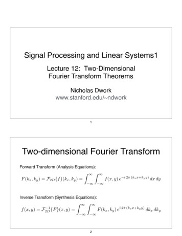
8.1Space, the Final Frontier339and the complex exponential is a function of t along the line:exp( 2πi x · ξ) exp( 2πi(aξ1 bξ2 )) exp( 2πitkξk) .The factor exp( 2πi(aξ1 bξ2 )) doesn’t depend on t and the factor exp( 2πitkξk) is periodic with period1/kξk, the spacing between the lines of zero phase. Now, if ξ1 or ξ2 is large, then the spacing of the lines isclose and, by the same token, if ξ1 and ξ2 are small then the lines are far apart. Thus although “frequency”is now a vector quantity we still tend to speak in terms of a “high frequency” harmonic, when the linesof zero phase are spaced close together and a “low frequency” harmonic when the lines of zero phase arespaced far apart (“high” and “low” are relatively speaking, of course). Half way between the lines of zerophase, when t 1/2kξk, we’re on lines where the exponential is 1, so 180 out of phase with the lines ofzero phase.One often sees pictures like the following.
340Chapter 8 n-dimensional Fourier TransformHere’s what you’re looking at: The function e2πix·ξ is complex valued, but consider its real part Re e2πix·ξ 21 e2πix·ξ e 2πix·ξ cos 2πix · ξ cos 2π(ξ1 x1 ξ2 x2 )which has the same periodicity and same lines of zero phase as the complex exponential. Put down whitestripes where cos 2π(ξ1 x1 ξ2 x2 ) 0 and black stripes where cos 2π(ξ1 x1 ξ2 x2 ) 0, or, if you want toget fancy, use a gray scale to go from pure white on the lines of zero phase, where the cosine is 1, down topure black on the lines 180 out of phase, where the cosine is 1, and back up again. This gives a senseof a periodically varying intensity, and the slowness or rapidity of the changes in intensity indicate low orhigh spatial frequencies.The spectrum The Fourier transform of a function f (x1 , x2 ) finds the spatial frequencies (ξ1 , ξ2 ). Theset of all spatial frequencies is called the spectrum, just as before. The inverse transform recovers thefunction from its spectrum, adding together the corresponding spatial harmonics, each contributing anamount Ff (ξ1 , ξ2 ). As mentioned above, when f (x1 , x2 ) is real we haveFf ( ξ1 , ξ2 ) Ff (ξ1 , ξ2 ) ,so that if a particular Ff (ξ1 , ξ2 ) is not zero then there is also a contribution from the “negative frequency”( ξ1 , ξ2 ). Thus for a real signal, the spectrum, as a set of points in the (ξ1 , ξ2 )-plane, is symmetric aboutthe origin.2 If we think of the exponentials of corresponding positive and negative frequency vectors addingup to give the signal then we’re adding up (integrating) a bunch of cosines and the signal really does seemto be made of a bunch of a stripes with different spacings, different orientations, and different intensities2N.b.: It’s not the values Ff (ξ1 , ξ2 ) that are symmetric, just the set of points (ξ1 , ξ2 ) of contributing frequencies.
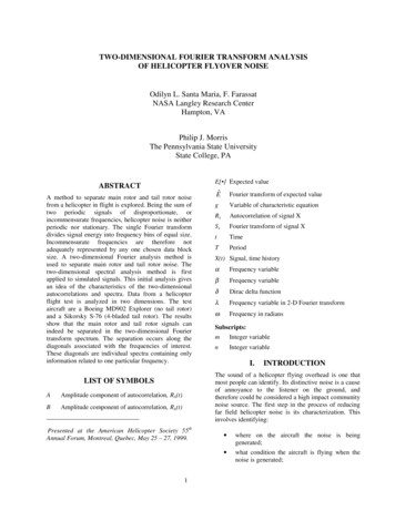
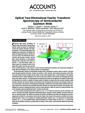
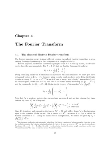
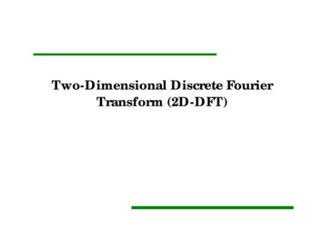
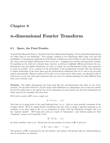
8.1Space, the Final Frontier341(the magnitudes Ff (ξ1 , ξ2 ) ). It may be hard to imagine that an image, for example, is such a sum ofstripes, but, then again, why is music the sum of a bunch of sine curves?In the one-dimensional case we are used to drawing a picture of the magnitude of the Fourier transformto get some sense of how the energy is distributed among the different frequencies. We can do a similarthing in the two-dimensional case, putting a bright (or colored) dot at each point (ξ1 , ξ2 ) that is in thespectrum, with a brightness proportional to the magnitude Ff (ξ1 , ξ2 ) . This, the energy spectrum or thepower spectrum, is symmetric about the origin because Ff (ξ1 , ξ2 ) Ff ( ξ1 , ξ2 ) .Here are pictures of the spatial harmonics we showed before and their respective spectra.Which is which? The stripes have an orientation (and a spacing) determined by ξ (ξ1 , ξ2 ) which is normalto the stripes. The horizontal stripes have a normal of the form (0, ξ2 ) and they are of lower frequency soξ2 is small. The vertical stripes have a normal of the form (ξ1 , 0) and are of a higher frequency so ξ1 islarge, and the oblique stripes have a normal of the form (ξ, ξ) with a spacing about the same as for thevertical stripesHere’s a more interesting example.3For the picture of the woman, what is the function we are taking the Fourier transform of ? The functionf (x1 , x2 ) is the intensity of light at each point (x1 , x2 ) — that’s what a black-and-white image is for thepurposes of Fourier analysis. Incidentally, because the dynamic range (the range of intensities) can be solarge in images it’s common to light up the pixels in the spectral picture according to the logarithm of theintensity.Here’s a natural application of filtering in the frequency domain for an image.The first picture shows periodic noise that appears quite distinctly in the frequency spectrum. We eliminatethose frequencies and take the inverse transform to show the plane more clearly.4Finally, there are reasons to add things to the spectrum as well as take them away. An important andrelatively new application of the Fourier transform in imaging is digital watermarking. Watermarking is anold technique to authenticate printed documents. Within the paper an image is imprinted (somehow — Idon’t know how this is done!) that only becomes visible if held up to a light or dampened by water. The3I showed this picture to the class a few years ago and someone yelled : “That’s Natalie!”4All of these examples are taken from the book Digital Image Processing by G. Baxes.
342Chapter 8 n-dimensional Fourier Transformidea is that someone trying to counterfeit the document will not know of or cannot replicate the watermark,but that someone who knows where to look can easily verify its existence and hence the authenticity of the
8.1Space, the Final Frontier343document. The newer US currency now uses watermarks, as well as other anticounterfeiting techniques.For electronic documents a digital watermark is added by adding to the spectrum. Insert a few extraharmonics here and there and keep track of what you added. This is done in a way to make the changes inthe image undetectable (you hope) and so that no one else could possibly tell what belongs in the spectrumand what you put there (you hope). If the receivers of the document know where to look in the spectrumthey can find your mark and verify that the document is legitimate.Higher dimensions In higher dimensions the words to describe the harmonics and the spectrum arepretty much the same, though we can’t draw the pictures5 . The harmonics are the complex exponentialse 2πix·ξ and we have n spatial frequencies, ξ (ξ1 , ξ2 , . . . , ξn ). Again we single out where the complexexponentials are equal to 1 (zero phase), which is when ξ · x is an integer. In three-dimensions a given(ξ1 , ξ2 , ξ3 ) defines a family ξ · x integer of parallel planes (of zero phase) in (x1 , x2 , x3 )-space. Thenormal to any of the planes is the vector ξ (ξ1 , ξ2 , ξ3 ) and adjacent planes are a distance 1/kξk apart.The exponential is periodic in the direction ξ with period 1/kξk. In a similar fashion, in n dimensionswe have families of parallel hyperplanes ((n 1)-dimensional “planes”) with normals ξ (ξ1 , . . . , ξn ), anddistance 1/kξk apart.8.1.2Finding a few Fourier transforms: separable functionsThere are times when a function f (x1 , . . . , xn ) of n variables can be written as a product of n functions ofone-variable, as inf (x1 , . . . , xn ) f1 (x1 )f2 (x2 ) · · · fn (xn ) .Attempting to do this is a standard technique in finding special solutions of partial differential equations— there it’s called the method of separation of variables. When a function can be factored in this way, itsFourier transform can be calculated as the product of the Fourier transform of the factors. Take n 2 asa representative case:Ze 2πix·ξ f (x) dxFf (ξ1 , ξ2 ) RnZ Z e 2πi(x1 ξ1 x2 ξ2 ) f (x1 , x2 ) dx1 dx2 Z Z e 2πiξ1 x1 e 2πiξ2 x2 f1 (x1 )f2 (x2 ) dx1 dx2 Z Z 2πiξ1 x1 ef1 (x) dx1 e 2πiξ2 x2 f2 (x2 ) dx2 Z e 2πiξ2 x2 f2 (x2 ) dx2 Ff1 (ξ1 ) Ff1 (ξ1 ) Ff2 (ξ2 )In general, if f (x1 , x2 , . . . , xn ) f1 (x1 )f2 (x2 ) · · · fn (xn ) thenFf (ξ1 , x2 , . . . ξn ) Ff1 (ξ1 )Ff2 (ξ2 ) · · · Ffn (ξn ) .If you really want to impress your friends and confound your enemies, you can invoke tensor products inthis context. In mathematical parlance the separable signal f is the tensor product of the functions fi and5Any computer graphics experts out there care to add color and 3D-rendering to try to draw the spectrum?
344Chapter 8 n-dimensional Fourier Transformone writesf f1 f2 · · · fn ,and the formula for the Fourier transform asF(f1 f2 · · · fn ) Ff1 Ff2 · · · Ffn .People run in terror from the symbol. Cool.Higher dimensional rect functions The simplest, useful example of a function that fits this descriptionis a version of the rect function in higher dimensions. In two dimensions, for example, we want the functionthat has the value 1 on the square of side length 1 centered at the origin, and has the value 0 outside thissquare. That is,(1 12 x1 21 , 21 x2 12Π(x1 , x2 ) 0 otherwiseYou can fight it out how you want to define things on the edges. Here’s a graph.We can factor Π(x1 , x2 ) as the product of two one-dimensional rect functions:Π(x1 , x2 ) Π(x1 )Π(x2 ) .(I’m using the same notation for the rect function in one or more dimensions because, in this case, there’slittle chance of confusion.) The reason that we can write Π(x1 , x2 ) this way is because it is identically1 if all the coordinates are between 1/2 and 1/2 and it is zero otherwise — so it’s zero if any of thecoordinates is outside this range. That’s exactly what happens for the product Π(x1 )Π(x2 ).
8.1Space, the Final Frontier345For the Fourier transform of the 2-dimensional Π we then haveFΠ(ξ1 , ξ2 ) sinc ξ1 sinc ξ2 .Here’s what the graph looks like.A helpful feature of factoring the rect function this way is the ability, easily, to change the widths in thedifferent coordinate directions. For example, the function which is 1 in the rectangle a1 /2 x1 a1 /2, a2 /2 x2 a2 /2 and zero outside that rectangle is (in appropriate notation)Πa1 a2 (x1 , x2 ) Πa1 (x1 )Πa2 (x2 ) .The Fourier transform of this isFΠa1 a2 (ξ1 , ξ2 ) (a1 sinc a1 ξ1 )(a2 sinc a2 ξ2 ) .Here’s a plot of (2 sinc 2ξ1 )(4 sinc 4ξ2 ). You can see how the shape has changed from what we had before.
346Chapter 8 n-dimensional Fourier TransformThe direct generalization of the (basic) rect function to n dimensions is(1 21 xk 12 , k 1, . . . , nΠ(x1 , x2 , . . . , xn ) 0 otherwisewhich factors asΠ(x1 , x2 , . . . , xn ) Π(x1 )Π(x2 ) · · · Π(xn ) .For the Fourier transform of the n-dimensional Π we then haveFΠ(ξ1 , ξ2 , . . . , ξn ) sinc ξ1 sinc ξ2 · · · sinc ξn .It’s obvious how to modify higher-dimensional Π to have different widths on different axes.Gaussians Another good example of a separable function — one that often comes up in practice — isa Gaussian. By analogy to the one-dimensional case, the most natural Gaussian to use in connection withFourier transforms is2222g(x) e π x e π(x1 x2 ··· xn ) .This factors as a product of n one-variable Gaussians:222222g(x1 , . . . , xn ) e π(x1 x2 ··· xn ) e πx1 e πx2 · · · e πxn h(x1 )h(x2 ) · · · h(xn ) ,where2h(xk ) e πxk .Taking the Fourier transform and applying the one-dimensional result (and reversing the algebra that wedid above) gets us2222222Fg(ξ) e πξ1 e πξ2 · · · e πξn e π(ξ1 ξ2 ··· ξn ) e π ξ .
8.2Getting to Know Your Higher Dimensional Fourier Transform347As for one dimension, we see that g is its own Fourier transform.Here’s a plot of the two-dimensional Gaussian.8.2Getting to Know Your Higher Dimensional Fourier TransformYou already know a lot about the higher dimensional Fourier transform because you already know a lotabout the one-dimensional Fourier transform — that’s the whole point. Still, it’s useful to collect a few ofthe basic facts. If some result corresponding to the one-dimensional case isn’t mentioned here, that doesn’tmean it doesn’t hold, or isn’t worth mentioning — it only means that the following is a very quick andvery partial survey. Sometimes we’ll work in Rn , for any n, and sometimes just in R2 ; nothing should beread into this for or against n 2.8.2.1LinearityLinearity is obvious:F(αf βg)(ξ) αFf (ξ) βFg(ξ) .8.2.2ShiftsIn one dimension a shift in time corresponds to a phase change in frequency. The statement of this is theshift theorem: If f (x) F (s) then f (x b) e 2πisb F (s).It looks a little slicker (to me) if we use the delay operator (τb f )(x) f (x b), for then we can writeF(τb f )(s) e 2πisb Ff (s) .
348Chapter 8 n-dimensional Fourier Transform(Remember, τb involves b.) Each to their own taste.The shift theorem in higher dimensions can be made to look just like it does in the one-dimensionalcase. Suppose that a point x (x1 , x2 , . . . , xn ) is shifted by a displacement b (b1 , b2 , . . . , bn ) tox b (x1 b1 , x2 b2 , . . . , xn bn ). Then the effect on the Fourier transform is: The Shift TheoremIf f (x) F (ξ) then f (x b) e 2πib·ξF (ξ).Vectors replace scalars and the dot product replaces multiplication, but the formulas look much the same.Again we can introduce the delay operator, this time “delaying” by a vector:τ b f (x) f (x b) ,and the shift theorem then takes the formF(τ b f )(ξ) e 2πib·ξFf (ξ) .(Remember, τ b involves a b.) Each to their own taste, again.If you’re more comfortable writing things out in coordinates, the result, in two dimensions, would read:Ff (x1 b1 , x2 b2 ) e2πi( ξ1 b1 ξ2 b2 ) Ff (ξ1 , ξ2 ) .The only advantage in writing it out this way (and you certainly wouldn’t do so for any dimension higherthan two) is a more visible reminder that in shifting (x1 , x2 ) to (x1 b1 , x2 b2 ) we shift the variablesindependently, so to speak. This independence is also (more) visible in the Fourier transform if we breakup the dot product and multiply the exponentials:Ff (x1 b1 , x2 b2 ) e 2πiξ1 b1 e 2πiξ2 b2 Ff (ξ1 , ξ2 ) .The derivation of the shift theorem is pretty much as in the one-dimensional case, but let me show youhow the change of variable works. We’ll do this for n 2, and, yes, we’ll write it out in coordinates. Let’sjust take the case when we’re adding b1 and b2 . First offZ Z F(f (x1 b2 , x2 b2 )) e 2πi(x1 ξ1 x2 ξ2 ) f (x1 b1 , x2 b2 ) dx1 dx2 We want to make a change of variable, turning f (x1 b1 , x2 b2 ) into f (u, v) by the substitutions u x1 b1and v x2 b2 (or equivalently x1 u b1 and x2 v b2 ). You have two choices at this point. Thegeneral change of variables formula for a multiple integral (stay with it for just a moment) immediatelyproduces.Z Z e 2πi(x1 ξ1 x2 ξ2 ) f (x1 b1 , x2 b2 ) dx1 dx2 Z Z e 2πi((u b1 )ξ1 (v b2 )ξ2 ) f (u, v) du dv Z Z e2πib1 ξ1 e2πib2 ξ2 e 2πi(uξ2 vξ2 ) f (u, v) du dv Z Z 2πi(b1 ξ1 b2 ξ2 ) ee 2πi(uξ2 vξ2 ) f (u, v) du dv 2πi(b1 ξ1 b2 ξ2 ) e Ff (ξ1 , ξ2 ) ,
8.2Getting to Know Your Higher Dimensional Fourier Transform349and there’s our formula.If you know the general change of variables formula then the shift formula and its derivation really are justlike the one-dimensional case, but this doesn’t do you much good if you don’t know the change of variablesformula for a multiple integral. So, for completeness, let me show you an alternative derivation that worksbecause the change of variables u x1 b1 , v x2 b2 changes x1 and x2 separately.Z Z Ff (x1 b2 , x2 b2 ) e 2πi(x1 ξ1 x2 ξ2 ) f (x1 b1 , x2 b2 ) dx1 dx2 Z Z 2πix1 ξ12πix2 ξ2eef (x1 b1 , x2 b2 ) dx2 dx1 Z Z 2πix1 ξ1 2πi(v b2 )ξ2eef (x1 b1 , v) dv dx1 (substituting v x2 b2 ) Z Z 2πib2 ξ2 2πivξ2 2πix1 ξ1 eeef (x1 b1 , v) dv dx1 Z Z 2πib2 ξ2 2πivξ2 2πix1 ξ1 eeef (x1 b1 , v) dx1 dv Z Z e 2πi(u b1 )ξ1 f (u, v) du dve 2πivξ2 e2πib2 ξ2 (substituting u x1 b1 ) Z Z e2πib2 ξ2 e2πib1 ξ1e 2πivξ2e 2πiuξ1 f (u, v) du dv Z Z e2πib2 ξ2 e2πib1 ξ1e 2πi(uξ1 vξ2 ) f (u, v) du dv e2πib2 ξ2 e2πib1 ξ1 Ff (ξ1 , ξ2 ) e2πi(b2 ξ2 b1 ξ1 ) Ff (ξ1 , ξ2 ) .And there’s our formula, again.The good news is, we’ve certainly derived the shift theorem! The bad news is, you may be saying to yourself:“This is not what I had in mind when you said the higher dimensional case is just like the one-dimensionalcase.” I don’t have a quick comeback to that, except that I’m trying to make honest statements about thesimilarities and the differences in the two cases and, if you want, you can assimilate the formulas and justskip those derivations in the higher dimensional case that bug your sense of simplicity. I will too, mostly.8.2.3StretchesThere’s really only one stretch theorem in higher dimensions, but I’d like to give two versions of it. Thefirst version can be derived in a manner similar to what we did for the shift theorem, making separatechanges of variable. This case comes up often enough that it’s worth giving it its own moment in thesun. The second version (which includes the first) needs the general change of variables formula for thederivation. Stretch Theorem, first version1F(f )F(f (a1 x1 , a2 x2 )) a1 a2 ξ1 ξ2,a1 a2 .
350Chapter 8 n-dimensional Fourier TransformThere is an analogous statement in higher dimensions.I’ll skip the derivation.The reason that there’s a second version of the stretch theorem is because there’s something new thatcan be done by way of transformations in higher dimensions that doesn’t come up in the one-dimensionalsetting. We can look at a linear change of variables in the spatial domain. In two dimensions we writethis as u1a bx1 u2c dx2or, written out,u1 ax1 bx2u2 cx1 dx2The simple, “independent” stretch is the special case a1 0x1u1. x20 a2u2For a general linear transformation the coordinates can get mixed up together instead of simply changingindependently.A linear change of coordinates is not at all an odd a thing to do — think of linearly distorting an image,for whatever reason. Think also of rotation, which we’ll consider below. Finally, a linear transformation asa linear change of coordinates isn’t much good if you can’t change the coordinates back. Thus it’s naturalto work only with invertible transformations here, i.e., those for which det A 6 0.The general stretch theorem answers the question of what happens to the spectrum when the spatialcoordinates change linearly — what is F(f (u1 , u2 )) F(f (ax1 bx2 , cx1 dx2 ))? The nice answer ismost compactly expressed in matrix notation, in fact just as easily for n dimensions as for two. Let A bean n n invertible matrix. We introduce the notationA T (A 1 )T ,the transpose of the inverse of A. You can check that also A T (AT ) 1 , i.e., A T can be defined eitheras the transpose of the inverse or as the inverse of the transpose. (A T will also come up naturally whenwe apply the Fourier transform to lattices and “reciprocal lattices”, i.e., to crystals.)We can now state: Stretch Theorem, general versionF(f (Ax)) 1Ff (A T ξ) . det A There’s another way of writing this that you might prefer, depending (as always) on your tastes. Usingdet AT det A and det A 1 1/ det A we have1 det A T det A so the formula readsF(f (Ax)) det A T Ff (A T ξ) .
8.2Getting to Know Your Higher Dimensional Fourier Transform351Finally, I’m of a mind to introduce the general scaling operator defined by(σA f )(x) f (Ax) ,where A is an invertible n n matrix. Then I’m of a mind to write1F(σA f )(ξ) Ff (A T ξ) . det A Your choice. I’ll give a derivation of the general stretch theorem in
n-dimensional Fourier Transform 8.1 Space, the Final Frontier To quote Ron Bracewell from p. 119 of his book Two-Dimensional Imaging, “In two dimensions phenomena are richer than in one dimension.” True enough, working in two dimensions offers many new and rich possibilities. Contempor