Transcription
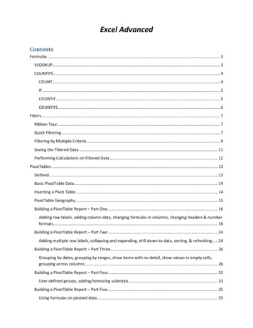
Excel AdvancedContentsFormulas . 3VLOOKUP. 3COUNTIFS . 4COUNT. 4IF . 5COUNTIF . 5COUNTIFS . 6Filters. 7Ribbon Tour. 7Quick Filtering . 7Filtering by Multiple Criteria . 9Saving the Filtered Data . 11Performing Calculations on Filtered Data . 12PivotTables . 13Defined. 13Basic PivotTable Data . 14Inserting a Pivot Table. 14PivotTable Geography . 15Building a PivotTable Report – Part One. 16Adding row labels, adding column data, changing formulas in columns, changing headers & numberformats . 16Building a PivotTable Report – Part Two . 24Adding multiple row labels, collapsing and expanding, drill down to data, sorting, & refreshing . 24Building a PivotTable Report – Part Three . 26Grouping by dates, grouping by ranges, show items with no detail, show values in empty cells,grouping across columns . 26Building a PivotTable Report – Part Four . 33User defined groups, adding/removing subtotals . 33Building a PivotTable Report – Part Five . 35Using formulas on pivoted data . 35
Building a PivotTable Report – Part Six . 37Displaying multiple row labels in columns, or tabular form. . 37Other Cool Things to do with a Pivot Table – Part Seven . 39Report Filters. 39Report Slicers . 40Expanding Filter Results to Individual Tabs . 41Formatting as a Table - Part Eight . 412
FormulasVLOOKUPThe VLOOKUP function searches vertically (top to bottom) the leftmost column of a table until a value thatmatches or exceeds the one you are looking up is found.The elements being looked up must be unique and must be arranged or sorted in ascending order; that is,alphabetical order for text entries, and lowest-to-highest order for numeric entries.The syntax is VLOOKUP(lookup value,table array,col index num,[range lookup]).An example of the formula is: VLOOKUP(E2,D2:M3,2,TRUE) The English translation is using the value found in thecell E2, look in the range of D2 to M3 row by row. If you find a value that matches or exceeds the value in E2,using that row, go over 2 columns to the right, grab the value there and bring it back.There are two range lookup argument options; TRUE or FALSETRUEIs the default answer, so you may leave it out of the formulaLooks for an approximate matchIf it finds an exact match it will use it.If it doesn’t find an exact match, it will use the last item before it got greaterAlphabetical: Looking for Cat. If elements are Apple, Bird, Carpet, Dog; then Carpetwould be returned because Dog exceeds Cat alphabetically.Numeric: Looking for 5.25. If elements are 3.0, 4.0, 5.0, 6.0, 7.0, then 5.0 would be used.The last number before 5.25 was exceeded.FALSELooks for an exact match.If it finds an exact match it will use it.If it doesn’t find an exact match, it will return #N/AAlphabetical: Looking for Cat. If elements are Apple, Bird, Carpet, Dog; then #N/A wouldbe returned.Numeric: Looking for 5.25. If elements are 3.0, 4.0, 5.0, 6.0, 7.0, then #N/A would bereturned because there is no exact match.3
COUNTIFSRecall quickly the COUNT and IF commands.COUNTThe COUNT function counts the number of cells that contain numbers and counts numbers within thelist of arguments.The syntax is COUNT( value1, value2, )Continuing on with our SUM formula from above, let’s not only add up the values of the range A1:A4,but let’s count how many numbers are included within the range, i.e. how many cells within the rangehas a value in it.The formula is COUNT(A1:A4). The English translation is count how many cells within the range has avalue in it and display the result.Notice that the range is exactly the same as ourSUM, A1:A4, which includes four rows. The valuereturned in cell A7 is three, because only three ofthe four rows have values in them.4
If you are trying to count text, use the COUNTA formula which counts the non-blank cells.IFThe formula makes a statement/question, if the answer is true then one response is obtained. If theanswer if false, then another answer is obtained.The syntax is IF(logical test,value if true,value if false)Continuing on with our SUM formula from above, let’s add some verbage to emphasize whether theresult is greater or less than twenty.The formula is if(A5 20,”Amount is less than twenty”,”Amount is more than twenty”). The Englishtranslation is if the value found in A5 is less than twenty THEN display the comment ‘Amount is less thantwenty’ ELSE display the comment ‘Amount is more than twenty’.COUNTIFThe COUNT function counts the number of cells in a range, that meets single criteria.5
COUNTIFSThe COUNT function counts the number of cells in a range that meets multiple criteria.6
FiltersRibbon TourQuick FilteringThe secret to filtering is not to have a space between your titles and your data. In fact, Excel is so smart, that youdo not even have your data selected, but may if you prefer.Select your data and left click onthe filter icon in the Sort & FilterGroup.Notice that a chevron appears tothe left of each header.7
By selecting the chevron to the left of Vendor Name, a dialogbox appears displaying all unique text filters found in the rangeas well as other common sort icons.If you only want a particular filter, deselect the (Select All) boxand check the filter you desire.In the below screen shot, Kendell Kilborn is selected. Notice the hidden rows to the left. Those representdata lines for mileage paid to individuals other than Kendell. No data is lost, it is just currently hidden.Also note that the icon to the left ofthe vendor name now displays the filter icon.This so at a glance the user may see that thedata range has been filtered.8
Filtering by Multiple CriteriaThe filtering tool is fine when you only want one item. However the power of the advance filter tool really shineswhen you want to sort by multiple criteria. There are several thou shalts of advanced filtering.Thou Shalts of Advanced Filtering1The headers in the criteria range must be exactly as they are in the list range2l must be at least one blank row between the criteria range and the list rangeThereSteps For Advanced Filtering1234567Create a criteria range by inserting a few rows and copying the header from the data range.Although not required, it is often best to have the range above your data for simplicity.Type in the criteria you want to filter by.Have your curser somewhere in the data rangeSelect the Advanced iconwith your left mouse button.The list range most likely will be your data. If not, you will need to correct it.Select your criteria range. The range must include the headers of the criteria range The rows with criteria All columns in the rangeSelect OK:9
415The results appear below.102
Saving the Filtered DataNow that the data has been filtered it would be great to save it so you can manipulate it further. To doso is a rather straight forward process. Basically you will go to where you want to save it, Sheet2 in ourexample, and go through the filtering process that we did above with just a couple of twists.Steps For Advanced FilteringOn the destination worksheet (Sheet2 for example) place the cursor in a blank cell.123Select the Advanced iconwith your left mouse button.Under Action, select copy to another location In the list range, select the range finder icon. Theappears. Navigate to the appropriateworksheet and select the data range not forgeting the headers, and click on thelittle icon at the bottom right.Do the same for the criteria range.For the copy to range, select the first cell and select OK411
4Performing Calculations on Filtered DataExcel’s traditional formulas do not work on filtered data since the function will be performed on boththe hidden and visible cells. To perform functions on filtered data one must use the subtotal function.The syntax is SUBTOTAL(function num, range reference1, range reference2, .)The following functionsmay be performed with the subtotal. The function num within the syntax relates to the M4MAX10VAR5MIN11VARP6PRODUCT12
An example of the formula is: SUBTOTAL(9,E12:F19) The English translation is using the ninthsubtotal function, which is SUM, add up all of the data within the range that is selected by the filter.For comparison, included is the SUM function for the same range which brought back the total for allof the data cells, hidden or displayed.PivotTablesDefinedThe foundation of what is a PivotTable report is explained as follows:As long as you can connect to the data, whether it be locally in the same workbook or remotelyin other locations, you can built PivotTable reports that rearrange the raw data and changeit into meaningful informationA pivot table is an interactive way to quickly summarize large amounts of data; to analyze numericaldata in detail and to answer unanticipated questions. They are especially designed for: Querying large amounts of data in many user-friendly waysSubtotaling and aggregating numeric data, summarizing data by categories and subcategories,and creating custom calculations and formulasExpanding and collapsing levels of data to focus your results, and drilling down to details fromthe summary data.Moving rows to columns or columns to rows (or “pivoting”0 to see different summaries of thesource data.Filtering, sorting, grouping, and conditionally formatting the most useful and interesting subsetof data to enable you to focus on the information that you want.13
Thou Shalts in PivotTable Land1Headers should be in columns, not rows2No blank rows between the headers and the data3Best to have the pivot table on a separate worksheet so it does not accidently clobber thedata4Best to have simple data, rows and columns of data.5Best to format your area as a table, especially when you will be adding data to it. The tableis automatically expanded when data is added to the next row. Now when you launchcreate a pivot table the range will be th
The syntax is IF(logical_test,value_if_true,value_if_false) Continuing on with our SUM formula from above, let’s add some verbage to emphasize whether the result is