Transcription
Mathematical Modeling and Statistical Methodsfor Risk ManagementLecture Notesc Henrik Hult and Filip Lindskog2007
Contents1 Some background to financial risk management1.1 A preliminary example . . . . . . . . . . . . . . . .1.2 Why risk management? . . . . . . . . . . . . . . .1.3 Regulators and supervisors . . . . . . . . . . . . .1.4 Why the government cares about the buffer capital1.5 Types of risk . . . . . . . . . . . . . . . . . . . . .1.6 Financial derivatives . . . . . . . . . . . . . . . . .11234442 Loss operators and financial portfolios2.1 Portfolios and the loss operator . . . . . . . . . . . . . . . . . . .2.2 The general case . . . . . . . . . . . . . . . . . . . . . . . . . . .667.3 Risk measurement113.1 Elementary measures of risk . . . . . . . . . . . . . . . . . . . . . 113.2 Risk measures based on the loss distribution . . . . . . . . . . . . 134 Methods for computing VaR and ES4.1 Empirical VaR and ES . . . . . . . . . . . . . . . . . . . .4.2 Confidence intervals . . . . . . . . . . . . . . . . . . . . .4.2.1 Exact confidence intervals for Value-at-Risk . . . .4.2.2 Using the bootstrap to obtain confidence intervals4.3 Historical simulation . . . . . . . . . . . . . . . . . . . . .4.4 Variance–Covariance method . . . . . . . . . . . . . . . .4.5 Monte-Carlo methods . . . . . . . . . . . . . . . . . . . .21212222242526265 Extreme value theory for random variables with heavy tails285.1 Quantile-quantile plots . . . . . . . . . . . . . . . . . . . . . . . . 285.2 Regular variation . . . . . . . . . . . . . . . . . . . . . . . . . . . 306 Hill estimation356.1 Selecting the number of upper order statistics . . . . . . . . . . . 367 The7.17.27.37.4Peaks Over Threshold (POT) methodHow to choose a high threshold. . . . . . . . . . . .Mean-excess plot . . . . . . . . . . . . . . . . . . .Parameter estimation . . . . . . . . . . . . . . . .Estimation of Value-at-Risk and Expected shortfall8 Multivariate distributions and dependence8.1 Basic properties of random vectors . . . . .8.2 Joint log return distributions . . . . . . . .8.3 Comonotonicity and countermonotonicity .8.4 Covariance and linear correlation . . . . . .8.5 Rank correlation . . . . . . . . . . . . . . .8.6 Tail dependence . . . . . . . . . . . . . . . .i.3839404143.45454646465052
9 Multivariate elliptical distributions9.1 The multivariate normal distribution . . . . .9.2 Normal mixtures . . . . . . . . . . . . . . . .9.3 Spherical distributions . . . . . . . . . . . . .9.4 Elliptical distributions . . . . . . . . . . . . .9.5 Properties of elliptical distributions . . . . . .9.6 Elliptical distributions and risk management10 Copulas10.1 Basic properties . . . . . . . . . . . . . . . . .10.2 Dependence measures . . . . . . . . . . . . .10.3 Elliptical copulas . . . . . . . . . . . . . . . .10.4 Simulation from Gaussian and t-copulas . . .10.5 Archimedean copulas . . . . . . . . . . . . . .10.6 Simulation from Gumbel and Clayton copulas10.7 Fitting copulas to data . . . . . . . . . . . . .10.8 Gaussian and t-copulas . . . . . . . . . . . . .11 Portfolio credit risk modeling11.1 A simple model . . . . . . . . . . . .11.2 Latent variable models . . . . . . . .11.3 Mixture models . . . . . . . . . . . .11.4 One-factor Bernoulli mixture models11.5 Probit normal mixture models . . . .11.6 Beta mixture models . . . . . . . . 2 Popular portfolio credit risk models9312.1 The KMV model . . . . . . . . . . . . . . . . . . . . . . . . . . . 9312.2 CreditRisk – a Poisson mixture model . . . . . . . . . . . . . . 97A A few probability facts105A.1 Convergence concepts . . . . . . . . . . . . . . . . . . . . . . . . 105A.2 Limit theorems and inequalities . . . . . . . . . . . . . . . . . . . 105B Conditional expectations106B.1 Definition and properties . . . . . . . . . . . . . . . . . . . . . . . 106B.2 An expression in terms the density of (X, Z) . . . . . . . . . . . 107B.3 Orthogonality and projections in Hilbert spaces . . . . . . . . . . 108ii
PrefaceThese lecture notes aim at giving an introduction to Quantitative Risk Management. We will introduce statistical techniques used for deriving the profitand-loss distribution for a portfolio of financial instruments and to compute riskmeasures associated with this distribution. The focus lies on the mathematical/statistical modeling of market- and credit risk. Operational risks and theuse of financial time series for risk modeling are not treated in these lecturenotes. Financial institutions typically hold portfolios consisting on large number of financial instruments. A careful modeling of the dependence betweenthese instruments is crucial for good risk management in these situations. Alarge part of these lecture notes is therefore devoted to the issue of dependencemodeling.The reader is assumed to have a mathematical/statistical knowledge corresponding to basic courses in linear algebra, analysis, statistics and an intermediatecourse in probability. The lecture notes are written with the aim of presentingthe material in a fairly rigorous way without any use of measure theory.The chapters 1-4 in these lecture notes are based on the book [12]which we strongly recommend. More material on the topics presented in remaining chapters can be found in [8] (chapters 5-7), [12](chapters 8-12) and articles found in the list of references at the endof these lecture notes.Henrik Hult and Filip Lindskog, 2007iii
1Some background to financial risk managementWe will now give a brief introduction to the topic of risk management andexplain why this may be of importance for a bank or financial institution. Wewill start with a preliminary example illustrating in a simple way some of theissues encountered when dealing with risks and risk measurements.1.1A preliminary exampleA player (investor/speculator) is entering a casino with an initial capital ofV0 1 million Swedish Kroner. All initial capital is used to place bets accordingto a predetermined gambling strategy. After the game the capital is V1 . Wedenote the profit(loss) by a random variable X V1 V0 . The distributionof X is called the profit-and-loss distribution (P&L) and the distribution ofL X V0 V1 is simply called the loss distribution. As the loss may bepositive this is a risky position, i.e. there is a risk of losing some of the initialcapital.Suppose a game is constructed so that it gives 1.6 million Swedish Kronerwith probability p and 0.6 million Swedish Kroner with probability 1 p. Hence, 0.6 with probability p,X (1.1) 0.4 with probability 1 p.The fair price for this game, corresponding to E(X) 0, is p 0.4. However,even if p 0.4 the player might choose not to participate in the game with theview that not participating is more attractive than playing a game with a smallexpected profit together with a risk of loosing 0.4 million Swedish Kroner. Thisattitude is called risk-averseness.Clearly, the choice of whether to participate or not depends on the P&Ldistribution. However, in most cases (think of investing in instruments on thefinancial market) the P&L distribution is not known. Then you need to evaluatesome aspects of the distribution to decide whether to play or not. For thispurpose it is natural to use a risk measure. A risk measure ̺ is a mappingfrom the random variables to the real numbers; to every loss random variableL there is a real number ̺(L) representing the riskiness of L. To evaluate theloss distribution in terms of a single number is of course a huge simplificationof the world but the hope is that it can give us sufficient indication whether toplay the game or not.Consider the game (1.1) described above and suppose that the mean E(L) 0.1 (i.e. a positive expected profit) and standard deviation std(L) 0.5 of theloss L is known. In this case the game had only two known possible outcomes sothe information about the mean and standard deviation uniquely specifies theP&L distribution, yielding p 0.5. However, the possible outcomes of a typicalreal-world game are typically not known and mean and standard deviation do1
not specify the P&L distribution. A simple example is the following: 0.35 with probability 0.8,X 0.9 with probability 0.2.(1.2)Here we also have E(L) 0.1 and std(L) 0.5. However, most risk-averseplayers would agree that the game (1.2) is riskier than the game (1.1) withp 0.5. Using an appropriate quantile of the loss L as a risk measure wouldclassify the game (1.2) as riskier than the game (1.1) with p 0.5. However,evaluating a single risk measure such as a quantile will in general not providea lot of information about the loss distribution, although it can provide somerelevant information. A key to a sound risk management is to look for riskmeasures that give as much relevant information about the loss distribution aspossible.A risk manager at a financial institution with responsibility for a portfolioconsisting of a few up to hundreds or thousands of financial assets and contractsfaces a similar problem as the player above entering the casino. Management orinvestors have also imposed risk preferences that the risk manager is trying tomeet. To evaluate the position the risk manager tries to assess the loss distribution to make sure that the current positions is in accordance with imposed riskpreferences. If it is not, then the risk manager must rebalance the portfolio untila desirable loss distribution is obtained. We may view a financial investor as aplayer participating in the game at the financial market and the loss distributionmust be evaluated in order to know which game the investor is participating in.1.2Why risk management?The trading volumes on the financial markets have increased tremendously overthe last decades. In 1970 the average daily trading volume at the New YorkStock Exchange was 3.5 million shares. In 2002 it was 1.4 billion shares. Inthe last few years we have seen a significant increase in the derivatives markets.There are a huge number of actors on the financial markets taking risky positionsContractsFOREXInterest rateTotal19951326471998185080200218102142Table 1: Global market in OTC derivatives (nominal value) in trillion US dollars(1 trillion 1012 ).and to evaluate their positions properly they need quantitative tools from riskmanagement. Recent history also shows several examples where large losses onthe financial market are mainly due to the absence of proper risk control.Example 1.1 (Orange County) On December 6 1994, Orange County, aprosperous district in California, declared bankruptcy after suffering losses of2
around 1.6 billion from a wrong-way bet on interest rates in one of its principalinvestment pools. (Source: www.erisk.com) Example 1.2 (Barings bank) Barings bank had a long history of success andwas much respected as the UK’s oldest merchant bank. But in February 1995,this highly regarded bank, with 900 million in capital, was bankrupted by 1billion of unauthorized trading losses. (Source: www.erisk.com) Example 1.3 (LTCM) In 1994 a hedge-fund called Long-Term Capital Management (LTCM) was founded and assembled a star team of traders and academics. Investors and investment banks invested 1.3 billion in the fund andafter two years returns was running close to 40%. Early 1998 the net assetvalue stands at 4 billion but at the end of the year the fund had lost substantial amounts of the investors equity capital and the fund was at the brinkof default. The US Federal Reserve managed a 3.5 billion rescue package toavoid the threat of a systematic crisis in th world financial system. (Source:www.erisk.com) 1.3Regulators and supervisorsTo be able to cover most financial losses most banks and financial institutionsput aside a buffer capital, also called regulatory capital. The amount of buffercapital needed is of course related to the amount of risk the bank is taking, i.e. tothe overall P&L distribution. The amount is regulated by law and the nationalsupervisory authority makes sure that the banks and financial institutions followthe rules.There is also a strive to develop international standards and methods forcomputing regulatory capital. This is the main task of the so-called Basel Committee. The Basel Committee, established in 1974, does not possess any formalsupernational supervising authority and its conclusions does not have legal force.It formulates supervisory standards, guidelines and recommends statements ofbest practice. In this way the Basel Committee has large impact on the nationalsupervisory authorities. In 1988 the first Basel Accord on Banking Supervision [2] initiated an important step toward an international minimal capital standard. Emphasiswas on credit risk. In 1996 an amendment to Basel I prescribes a so–called standardized modelfor market risk with an option for larger banks to use internal Value-atRisk (VaR) models. In 2001 a new consultative process for the new Basel Accord (Basel II)is initiated. The main theme concerns advanced internal approaches tocredit risk and also new capital requirements for operational risk. The newAccord aims at an implementation date of 2006-2007. Details of Basel IIis still hotly debated.3
1.4Why the government cares about the buffer capitalThe following motivation is given in [6].“Banks collect deposits and play a key role in the payment system. Nationalgovernments have a very direct interest in ensuring that banks remain capableof meeting their obligations; in effect they act as a guarantor, sometimes alsoas a lender of last resort. They therefore wish to limit the cost of the safetynet in case of a bank failure. By acting as a buffer against unanticipated losses,regulatory capital helps to privatize a burden that would otherwise be borne bynational governments.”1.5Types of riskHere is a general definition of risk for an organization: any event or action thatmay adversely affect an organization to achieve its obligations and execute itsstrategies. In financial risk management we try to be a bit more specific anddivide most risks into three categories. Market risk – risks due to changing markets, market prices, interest ratefluctuations, foreign exchange rate changes, commodity price changes etc. Credit risk – the risk carried by the lender that a debtor will not be ableto repay his/her debt or that a counterparty in a financial agreement cannot fulfill his/her commitments. Operational risk – the risk of losses resulting from inadequate of failedinternal processes, people and systems of from external events. This includes people risks such as incompetence and fraud, process risk such astransaction and operational control risk and technology risk such as system failure, programming errors etc.There are also other types of risks such as liquidity risk which is risk thatconcerns the need for well functioning financial markets where one can buy orsell contracts at fair prices. Other types of risks are for instance legal risk andreputational risk.1.6Financial derivativesFinancial derivatives are financial products or contracts derived from some fundamental underlying; a stock price, stock index, interest rate, commodity priceto name a few. The key example is the European Call option written on aparticular stock. It gives the holder the right but not the obligation at a givendate T to buy the stock S for the price K. For this the buyer pays a premiumat time zero. The value of the European Call at time T is thenC(T ) max(ST K, 0).Financial derivatives are traded not only for the purpose of speculation but isactively used as a risk management tool as they are tailor made for exchanging4
risks between actors on the financial market. Although they are of great importance in risk management we will not discuss financial derivatives much in thiscourse but put emphasis on the statistical models and methods for modelingfinancial data.5
2Loss operators and financial portfoliosHere we follow [12] to introduce the loss operator and give some examples offinancial portfolios that fit into this framework.2.1Portfolios and the loss operatorConsider a given portfolio such as for instance a collection of stocks, bonds orrisky loans, or the overall position of a financial institution.The value of the portfolio at time t is denoted V (t). Given a time horizon t the profit over the interval [t, t t] is given by V (t t) V (t) and thedistribution of V (t t) V (t) is called the profit-and-loss distribution (P&L).The loss over the interval is thenL[t,t t] (V (t t) V (t))and the distribution of L[t,t t] is called the loss distribution. Typical valuesof t is one day (or 1/250 years as we have approximately 250 trading days inone year), ten days, one month or one year.We may introduce a discrete parameter n 0, 1, 2, . . . and use tn n t asthe actual time. We will sometimes use the notationLn 1 L[tn ,tn 1 ] L[n t,(n 1) t] (V ((n 1) t) V (n t)).Often we also write Vn for V (n t).Example 2.1 Consider a portfolio of d stocks with αi units of stock number i,i 1, . . . , d. The stock prices at time n are given by Sn,i , i 1, . . . , d, and thevalue of the portfolio isVn dXαi Sn,i .i 1In financial statistics one often tries to find a statistical model for the evolutionof the stock prices, e.g. a model for Sn 1,i Sn,i , to be able to compute theloss distribution Ln 1 . However, it is often the case that the so-called logreturns Xn 1,i ln Sn 1,i ln Sn,i are easier to model than the differencesSn 1,i Sn,i . With Zn,i ln Sn,i we have Sn,i exp{Zn,i } so the portfolio lossLn 1 (Vn 1 Vn ) may be written asLn 1 dXi 1dXi 1dXi 1αi (exp{Zn 1,i } exp{Zn,i })αi exp{Zn,i }(exp{Xn 1,i } 1)αi Sn,i (exp{Xn 1,i } 1).6
The relation between the modeled variables Xn 1,i and the loss Ln 1 is nonlinear and it is sometimes useful to linearize this relation. In this case this is doneby replacing ex by 1 x; recall the Taylor expansion ex 1 x O(x2 ). Thenthe linearized loss is given byL n 1 dXαi Sn,i Xn 1,i .i 1 2.2The general caseA general portfolio with value Vn is often modeled using a d-dimensional randomvector Zn (Zn,1 , . . . , Zn,d ) of risk-factors. The value of the portfolio is thenexpressed asVn f (tn , Zn )for some known function f and tn is the actual calendar time. As in the exampleabove it is often convenient to model the risk-factor changes Xn 1 Zn 1 Zn .Then the loss is given by Ln 1 (Vn 1 Vn ) f (tn 1 , Zn Xn 1 ) f (tn , Zn ) .The loss may be viewed as the result of applying an operator l[n] (·) to therisk-factor changes Xn 1 so thatLn 1 l[n] (Xn 1 )where l[n] (x) f (tn 1 , Zn x) f (tn , Zn ) .The operator l[n] (·) is called the loss-operator. If we want to linearize the relationbetween Ln 1 and Xn 1 then we have to differentiate f to get the linearizedlossL n 1 ft (tn , Zn ) t dXi 1 fzi (tn , Zn )Xn 1,i .Here ft (t, z) f (t, z)/ t and fzi (t, z) f (t, z)/ zi. The correspondingoperator given by l[n](x) ft (tn , Zn ) t is called the linearized loss-operator.7dXi 1fzi (tn , Zn )xi
Example 2.2 (Portfolio of stocks continued) In the previous example of aportfolio of stocks the risk-factors are the log-prices of the stocks Zn,i ln Sn,iand the risk-factor-changes are the log returns Xn 1,i ln Sn 1,i ln Sn,i . The loss is Ln 1 l[n] (Xn 1 ) and the linearized loss is L n 1 l[n] (Xn 1 ), wherel[n] (x) dXi 1αi Sn,i (exp{xi } 1)and l[n](x) dXαi Sn,i xii 1are the loss operator and linearized loss operator, respectively. The following examples may convince you that there are many relevant examples from finance that fits into this general framework of risk-factors andloss-operators.Example 2.3 (A bond portfolio) A zero-coupon bond with maturity T is acontract which gives the holder of the contract 1 at time T . The price of thecontract at time t T is denoted B(t, T ) and by definition B(T, T ) 1. To azero-coupon bond we associate the continuously compounded yieldy(t, T ) 1ln B(t, T ),T ti.e.B(t, T ) exp{ (T t)y(t, T )}.To understand the notion of the yield, consider a bank account where we get aconstant interest rate r. The bank account evolves according to the differentialequationdSt rSt ,dtS0 1which has the solution St exp{rt}. This means that in every infinitesimal timeinterval dt we get the interest rate r. Every dollar put into the bank accountat time t is then worth exp{r(T t)} dollars at time T . Hence, if we haveexp{ r(T t)} dollars on the account at time t then we have exactly 1 at timeT . The yield y(t, T ) can be identified with r and is interpreted as the constantinterest rate contracted at t that we get over the period [t, T ]. However, theyield may be different for different maturity times T . The function T 7 y(t, T )for fixed t is called the yield-curve at t. Consider now a portfolio consisting ofd different (default free) zero-coupon bonds with maturity times Ti and pricesB(t, Ti ). We suppose that we have αi units of the bond with maturity Ti sothat the value of the portfolio isVn dXαi B(tn , Ti ).i 18
It is natural to use the yields Zn,i y(tn , Ti ) as risk-factors. ThenVn dXi 1αi exp{ (Ti tn )Zn,i } f (tn , Zn )and the loss is given by (with Xn 1,i Zn 1,i Zn,i and t tn 1 tn )Ln 1 dXi 1dXi 1 αi exp{ (Ti tn 1 )(Zn,i Xn 1,i )} exp{ (Ti tn )Zn,i } αi B(tn , Ti ) exp{Zn,i t (Ti tn 1 )Xn 1,i } 1 . The corresponding loss-operator is thenl[n] (x) dXi 1 αi B(tn , Ti ) exp{Zn,i t (Ti tn 1 )xi } 1 and the linearized loss is given byL n 1 dXi 1 αi B(tn , Ti ) Zn,i t (Ti tn 1 )Xn 1,i . Example 2.4 (European call and put) In this example we will consider aportfolio consisting of one European call or put option on a nondividend payingstock with price St for one share at time t, with maturity date T t and strikeprice K. A European call option is a contract which pays max(ST K, 0) tothe holder of the contract at time T . A European put option pays the holdermax(K ST , 0) at time T . The price at time t T for the contract is evaluatedusing a function C (for call) or P (for put) depending on some parameters.In the Black-Scholes model C C(t, T, St , K, r, σ) and P P (t, T, St , K, r, σ),where the time to maturity T t is measured in years, r is the continuouslycompounded interest rate per year and σ is the volatility (corresponding to thestandard deviation of the one-year log return for the stock price). We haveC(t, T, St , K, r, σ) St Φ(d1 ) Ke r(T t) Φ(d2 ),P (t, T, St, K, r, σ) Ke r(T t) Φ( d2 ) St Φ( d1 ), ln(St /K) (r σ 2 /2)(T t) d1 , d2 d1 σ T t.σ T tIn this case with time measured in years we may set t tn n t and T tn k (n k) t, where t 1/250 years (approximately 250 trading days peryear). In this case we may putZn (ln Sn , rn , σn )Xn 1 (ln Sn 1 ln Sn , rn 1 rn , σn 1 σn ).9
The value of the portfolio is Vn C(tn , T, Sn , K, rn, σn ) for the call option andVn P (tn , T, Sn , K, rn, σn ) for the put option. The linearized loss is given byL n 1 (Ct t CS Xn 1,1 Cr Xn 1,2 Cσ Xn 1,3 ),L n 1 (Pt t PS Xn 1,1 Pr Xn 1,2 Pσ Xn 1,3 )for the call and put option, respectively. The partial derivatives are usuallycalled the “Greeks”. Ct is called theta; CS is called delta; Cr is called rho; Cσis called vega (although this is not a Greek letter). 10
3Risk measurementWhat is the purpose of risk measurement? Determination of risk capital – determine the amount of capital a financialinstitution needs to cover unexpected losses. Management tool – Risk measures are used by management to limit theamount of risk a unit within the firm may take.Next we present some common measures of risk.3.1Elementary measures of riskNotional amountRisk of a portfolio is measured as the sum of notional values of individual securities, weighted by a factor for each asset class. The notional amount approachis used for instance in the standard approach of the Basel Committee where riskweights 0%, 10%, 20%, 50% and 100% are used (see [2]). Then the regulatorycapital should be such thatregulatory capital 8%.risk-weighted sumExample 3.1 Suppose we have a portfolio with three claims each of notionalamount 1 million. The first claim is on an OECD central bank, the second ona multilateral developed bank and the third on the private sector. According tothe risk-weights used by the Basel document the first claim is weighted by 0%,the second by 20% and the third by 100%. Thus the risk-weighted sum is0 106 0.20 106 1 106 1 200 000,and the regulatory capital should be at least 8% of this amount, i.e. 96 000. Advantage: easy to use.Disadvantage: Does not differentiate between long and short positions. Thereare no diversification effects; a portfolio with loans to m independent obligorsis considered as risky as the same amount lent to a single obligor.Factor sensitivity measuresFactor sensitivity measures gives the change in portfolio value for a predetermined change in one of the underlying risk factors. If the value of the portfoliois given byVn f (tn , Zn )then factor sensitivity measures are given by the partial derivativesfzi (tn , Zn ) f(tn , Zn ). zi11
The “Greeks” of a derivative portfolio may be considered as factor sensitivitymeasures.Advantage: Factor sensitivity measures provide information about the robustness of the portfolio value with respect to certain events (risk-factor changes).Disadvantage: It is difficult to aggregate the sensitivity with respect to changesin different risk-factors or aggregate across markets to get an understanding ofthe overall riskiness of a position.Scenario based risk measuresIn this approach we consider a number of possible scenarios, i.e. a number ofpossible risk-factor changes. A scenario may be for instance a 10% rise in arelevant exchange rate and a simultaneous 20% drop in a relevant stock index.The risk is then measured as the maximum loss over all possible (predetermined)scenarios. To assess the maximum loss extreme scenarios may be down-weightedin a suitable way.Formally, this approach may be formulated as follows. Fix a number Nof possible risk-factor changes, X {x1 , x2 , . . . , xN }. Each scenario is givena weight, wi and we write w (w1 , . . . , wN ). We consider a portfolio withloss-operator l[n] (·). The risk of the portfolio is then measured asψ[X,w] max{w1 l[n] (x1 ), . . . , wN l[n] (xN )}These risk measures are frequently used in practice (example: Chicago Mercantile Exchange).Example 3.2 (The SPAN rules) As an example of a scenario based riskmeasure we consider the SPAN rules used at the Chicago Mercantile Exchange[1]. We describe how the initial margin is calculated for a simple portfolio consisting of units of a futures contract and of several puts and calls with a commonexpiration date on this futures contract. The SPAN margin for such a portfoliois compute as follows: First fourteen scenarios are considered. Each scenariois specified by an up or down move of volatility combined with no move, or anup move, or a down move of the futures prices by 1/3, 2/3 or 3/3 of a specific“range”. Next, two additional scenarios relate to “extreme” up or down movesof the futures prices. The measure of risk is the maximum loss incurred, usingthe full loss of the first fourteen scenarios and only 35% of the loss for the lasttwo “extreme” scenarios. A specified model, typically the Black model, is usedto generate the corresponding prices for the options under each scenario.The account of the investor holding a portfolio is required to have sufficientcurrent net worth to support the maximum expected loss. If it does not, thenextra cash is required as margin call, an amount equal to the “measure of risk”involved. Loss distribution approachThis is the approach a statistician would use to compute the risk of a portfolio.Here we try model the loss Ln 1 using a probability distribution FL . The12
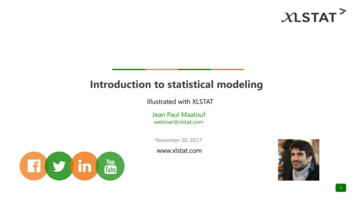
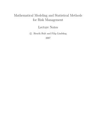
parameters of the loss distribution are estimated using historical data. One caneither try to model the loss distribution directly or to model the risk-factorsor risk-factor changes as a d-dimensional random vector or a multivariate timeseries. Risk measures are based on the distribution function FL . The nextsection studies this approach to risk measurement.3.2Risk measures based on the loss distributionStandard deviationThe standard deviation of the loss distribution as a measure of risk is frequentlyused, in particular in portfolio theory. There are however some disadvantagesusing the standard deviation as a measure of risk. For instance the standarddeviation is only defined for distributions with E(L2 ) , so it is undefined forrandom variables with very heavy tails. More important, profits and losses haveequal impact on the standard deviation as risk measure and it does not discriminate between distributions with apparently different probability of potentiallylarge losses. In fact, the standard deviation does not provide any informationon how large potential losses may be. 5051510log .0300.03520Example 3.3 Consider for instance the two loss distributions L1 N(0, 2)and L2 t4 (standard Student’s t-distribution with 4 degrees of freedom).Both L1 and L2 have standard deviation equal to 2. The probability densityis illustrated in Figure 1 for the two distributions. Clearly the probability oflarge losses is much higher for the t4 than for the
cal/statistical modeling of market- and credit risk. Operational risks and the use of financial time series for risk modeling are not treated in these lecture notes. Financial institutions typically hold portfolios consisting on large num-ber of financial