Transcription
Structural Mechanics2.080 Lecture 5Semester YrLecture 5: Solution Method for Beam Deflections5.1Governing EquationsSo far we have established three groups of equations fully characterizing the response ofbeams to different types of loading. In Lecture 2 relations were established to calculatestrains from the displacement field. (x, z) (x) zκ(5.1)where d2 wdu 1 dw 2 , κ 2(5.2) (x) dx 2 dxdxThe above geometrical relation are independent on equilibrium and apply to any kind ofmaterials.The second set of equations, derived in Lecture 3, is the equilibrium requirement dV q(x) 0 force equilibrium(5.3)dxdM V 0 moment equilibrium(5.4)dxdwwhere V V Nis the effective shear.(5.5)dxdN 0(5.6)dxEliminating V and V between the above equations, the beam equilibrium equation wasobtained (See Eq. (3.74))d2 wd2 M N q 0(5.7)dx2dx2The derivation of the equilibrium is valid for all types of materials. In the theory ofmoderately large deflections, the equilibrium is coupled with the kinematics.The third group of equation define the material behavior and relates the generalizedstrains to generalized forcesN EA (5.8)M EIκ(5.9)Independence of geometry and equilibrium on constitutive equation allows to develop thegeneral framework of a solver in the Finite Element codes. The constitutive equations canthen be added as a user Defined Subroutines.Let’s consider first the infinitesimal deformations (small rotations for which the term 1 dw 2d2 wvanish in Eq. (5.2) and the term 0 in Eq. (5.7). Then from Eqs. (5.2,2 dxdx25.4 and 5.8) one obtainsd2 u(5.10)EA 2 0dx5-1
Structural Mechanics2.080 Lecture 5Semester YrEliminating the curvature and bending moments between Eqs. (5.2, 5.7 and 5.9), the beamdeflection equation is obtainedd4 w(5.11)EI 4 q(x)dxThe concentrated load P can be treated as a special case of the distributed load q(x) P δ(x x0 ), where δ is the Dirac delta function.Let’s consider first Eq. (5.4) for the axial displacement. The boundary conditions inthe x-direction are(N N̄ )δu 0(5.12)The general solution for u(x) isdu D1 , u D1 x D0dx(5.13)There are two integration constants, and two boundary conditions are needed. There areonly four combinations of boundary conditions:1. Beam restricted from axial motion, see Fig. (5.1).u(x 0) u(x l) 0(5.14)This gives rise to the solution of two algebraic equation0 D0 D1 · 00 D0 D1 l(5.15a)(5.15b)which gives D0 D1 0 and u(x) 0. This is a trivial case, for which the axialduvanishes as well.force N EAdxxu 0u 0 Fixed(Kinematic)N 0N 0 Sliding(Static)N 0u 0 MixedFigure 5.1: Three combinations of in-plane boundary conditions for u(x).5-2
Structural Mechanics2.080 Lecture 5Semester Yr2. Beam allowed to slide in the x-direction on both ends.N̄ N 0at x 0 and x l(5.16)du. From Eq. (5.13) we can see that the gradientdxduof u is zero along the entire beam. So, if N̄ 0 orvanishes at one end, say x 0,dxD1 0 and automatically N̄ 0 is satisfied at the other end, x l. The integrationconstant D0 is undetermined meaning that the rigid body translation of the entirebeam is allowed.The axial force is proportional to3. In order to prevent the rigid body translation, one end of the beam, say x 0, mustbe fixed against motion in the x-direction. ThusN̄ 0 ordu 0dxu 0atx 0(5.17a)atx l(5.17b)which are precisely the boundary conditions for the third case. From Eq. (5.13) wegetD1 0(5.18a)D1 l D2 0 D2 0(5.18b)Now, the axial displacement vanishes, u(x) 0 but the rigid body translation iseliminated.For all the above three cases of kinematic static and mixed boundary conditions, theaxial force was zero.4. If one end of the beam (bar) is loaded by a given force N̄ and the other one is fixed,the boundary conditions (BC) areN N̄ , EAdu 0dxu 0at x 0(5.19)at x lD1 N̄N̄ l, D2 EAEA(5.20)N̄(l x)EA(5.21)and the solution isu(x) The case in which the nonlinear term is retained in Eq. (5.2) is much more interesting.This will be dealt with in the section on moderately large deflection of beams.5-3
Structural Mechanics2.080 Lecture 5Semester YrWe now turn our attention to the solution of the beam deflection, Eq. (5.11). This isthe fourth-order linear inhomogeneous equation which requires four boundary conditions.There are four types of boundary conditions, defined by(M M̄ )δw0 0(5.22a)(V V̄ )δw 0(5.22b)For the sake of illustration, we select a pin-pin BC for a beam loaded by the uniformlike load q, Fig. (5.2).Figure 5.2: Pin support allows for rotation but not for vertical translation.The bending moment is proportional to the curvature. Eq. (5.11) is then subjected tothe following boundary conditions:w(x 0) w(x l) 0d2 wdx2 x 0d2 wdx2 0(5.23a)(5.23b)x lLet’s integrate the differential equation four times with respect to x:d3 wdx3d2 wdx2dwdxdwdxqx C1EAqx2 C1 x C2EA2qx3C1 x 2 C2 x C3EA62qx4C1 x3 C2 x2 C3 x C4EA2462 (5.24a)(5.24b)(5.24c)(5.24d)Substituting the BC into the general solutions, one gets0 C2(5.25a)ql3 C1 l C22EA0 C40 0 ql4C1 l 3 C2 l 2 C3 l C424EA625-4(5.25b)(5.25c)(5.25d)
Structural Mechanics2.080 Lecture 5Semester YrThe solution of the above system isC1 ql2C2 0ql312C4 0C3 (5.26a)(5.26b)(5.26c)(5.26d)The load-displacement relation becomesw(x) qx(l3 2lx2 x3 )24EA(5.27)Differentiating Eq. (5.27) twice, the expression for the bending moment isM (x) qx(l x)2(5.28)and differentiating again, the shear force becomesV (x) qdM (l 2x)dx2(5.29)Plots of the normalized bending moments and shear forces are shown in Fig. (5.3).Figure 5.3: Parabolic distribution of the bending moment and linear variation of the shearforce.d3 wThe shear force V EI 3 is seen to vanish at the mid-span of the beam. Also thedxdwslopeis zero at this location. We have proved that at the symmetry planedxlV (x ) 02dw 0dx x l(5.30a)(5.30b)2Inversely, if the problem is symmetric, that Eq. (5.30) must hold at the symmetry plane.As an alternative formulation, one can consider a half of the beam with the symmetry BC.Can you solve the above problem and compare it with solution of the pin-pin beam, Eq.(5.27)?5-5
Structural Mechanics2.080 Lecture 5Semester Yrl/2M 0w 0V 0dw 0dxxFigure 5.4: Simply-supported plate with symmetry boundary conditions.It should be mentioned that the pin-pin supported beam is a statically determinatestructure. Therefore the distribution of shear forces and bending moments can be determined from the equilibrium equation alone. Can you do it and get correctly the signs?The purpose of Lecture 5 is to present properties of the governing equations and solutions. interested students are referred to end chapter of problem sets where many beamswith different loading and BC are considered. Also the recommended reference book andmonographs present solution to some common beam problems.5.2General Properties of the Beam Governing Equation:General and Particular SolutionsRecall from the Calculus that solution of the inhomogeneous, linear ordinary differentialequation is a sum of the general solution of the homogeneous equation wg and the particularsolution of the inhomogeneous equation wp . The property of homogeneity means thatf (Ax) Af (x). The homogeneous counterpart of Eq. (5.11) isd4 wd4 w 0or 0dx4dx4and its solution, obtained by four integrations is the third order polynomialEI(5.31)C1 x 3 C2 x 2 C3 x C4(5.32)62The particular solution wp of the beam deflection equation, Eq. (5.11) depends on theloading, but not the boundary conditions. For the uniformly loaded beam the particularsolution is the first term in Eq. (5.23d). As an illustration, consider the same pin-pinsupported beam loaded by the triangular line loadwg (x) 2xl, 0 x (5.33)l2where q0 is the load intensity at mid-span x l/2. The particular solution of this problem,satisfying the governing equation isq(x) q0wp q0 x560EIl5-6(5.34)
Structural Mechanics2.080 Lecture 5Semester YrThen, the full solution is w(x) wg wp .Beam loaded by concentrated forces (or moments) requires special consideration.Continuity requirementsA sudden change in the beam cross-section or loading may produce a discontinuous solution.What quantities may suffer a jump and what must be continuous?wFigure 5.5: The displacement and slope discontinuities are not allowed in beams.In mechanics the discontinuity of a given function is denoted by a square bracket[f (ξ)] f (ξ ) f (ξ )(5.35)where ξ and ξ denote the values of the argument on the right and left hand of a discontinuity. In the quasi-static theory of beam [w] 0 dw 0dx(5.36a)(5.36b)The discontinuity in the vertical displacement means separation so of course it may notoccur. Why then slopes must be continuous for elastic beams? This is simple. A changeof slope is called a curvature. A jump in the slope gives an infinite curvature, and thus aninfinite bending moments. Such a situation is impossible, because the beam cross-sectionwill go into plastic range, and the beam will no longer stay elastic. Quantities that can bediscontinuous areBending monents[M ] M̄(5.37a)Shear force[V ] V̄(5.37b)As an illustration, consider a pin-pin supported beam loaded at mid-span by a pointforce P .As mentioned earlier, the point load can be considered as a limiting case of a continuousline load with the help of the Dirac delta functionZll(5.38)q(x) P δ(x ), where δ(x )dx 122Even though techniques have been developed to deal with singularity functions forbeams, they require to use the apparatus of the mathematical theory of distribution. This5-7
Structural Mechanics2.080 Lecture 5Semester YrP2Pw 0M 0w 0M 0w 0M 0l/2xPV 2dw 0dxFigure 5.6: Symmetric loading of a beam by a concentrated force.is not the avenue that we will take. instead, a symmetry boundary condition will be imposed. Now, the concentrated load is not applied inside the beam 0 x l, governed bythe inhomogeneous differential equation, but at the boundary. Each half of the beam iscarrying half of the load. Therefore, the boundary conditions areat x 0 w 0d2 wdx2at x l2(5.39a) 0(5.39b)P2(5.39c)V dw 0dx(5.39d)Because the loading is applied on the boundary, the differential equation becomes homogeneous. The solution of Eq. (5.31) is given by the third order polynomial, substituting theabove BC into the solution given by Eq. (5.32), a system of four linear algebraic equationsis obtained, where the solution isC1 DP l2, C2 0, C3 , C4 02EI16EI(5.40)Px(3l2 4x2 )48EI(5.41)The deflection line is given byw(x) and the central deflection (something to remember) islpl3w0 w(x ) 248EI(5.42)The plot of the distribution of bending moment and shear forces along the length of thebeam determined from the calculated deflection line is shown in Fig. (5.7).Note that the jump in the internal shear force is equal to the applied forcell[V ] Vright (x ) Vleft (x ) P225-8(5.43)
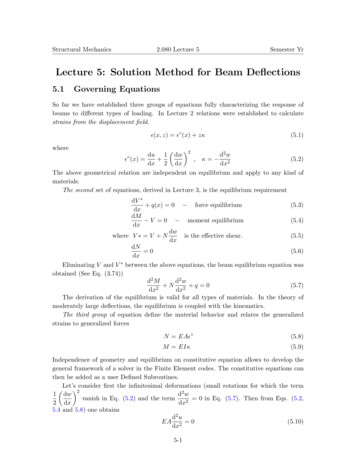
Structural Mechanics2.080 Lecture 5P2PSemester YrV(x)P2M(x)Figure 5.7: Bending moment is continuous at the mid-span, but the shear force is not.If the point load is not applied at the mid-span but at an arbitrary distance x a, thebeam must be divided into two parts 0 x a, a x l, and each part must be solvedindependently.First segment 0 x aSecond segment a x lC1 x 3 C2 x 2 C3 x C462C5 x 3 C6 x 2wII (x) C7 x C862wI (x) (5.44a)(5.44b)This gives rise to eight integration constants, four for each side. Would there be enoughconditions to determine these constants? The answer is YES.There are two boundaryconditions at x 0, four continuity conditions at x a, given by Eqs. (5.36-5.37) and,again, two boundary conditions at x l. In summaryBC, x 0w 0M 0Continuity, x a[w] 0dw 0dx[M ] 0[V ] PBC, x lw 0M 0(5.45)Note that there is no concentrated bending moment applied M̄ 0 so that the bendingmoment field is continueous across x a. The concentrated force produces a jump in thedistribution of the shear forces, so V̄ P .We leave it to the reader to apply the above condition and solve the problem. More onthis problem can be found in two sections of this notes: Problem Sets and Recitations.The method of superposition says that the deflections and slopes of the beam subjectedto a system of loads are equal to the sum of those quantities due to individual loads. Inother words the individual results may be superimposed to determine a combined response,hence the term method of superposition.This is a very powerful and convenient method since solutions for many support and loading conditions are readily available in various engineering handbooks. Using the principleof superposition, we may combine these solutions to obtain a solution for more complicatedloading conditions.As an example, consider a clamped-clamped beam loaded by a uniform line load q andconcentrated force at the center P . The deflection formulas for the two individual loading5-9
Structural Mechanics2.080 Lecture 5Semester Yrareqx2(l x)224EIP x2w point (3l 4x)48EIThe solution for both loads acting together isw uniform wtotal w uniform w point5.3(5.46a)(5.46b)(5.47)Statically Determined BeamsBeam for which the distribution of bending moments and shear forces can be determinedfrom the equilibrium alone are called statically determinate beams. For such beams M (x)and V (x) are known and determination of beam deflection will be a much easier task.Combining Eq. (5.9) with Eq. (5.2) one ends up with the following second order lineardifferential equationd2 w EI 2 M (x)(5.48)dxThe bending moment, which by itself should satisfy the second order differential equation, Eq. (5.7) should now obey two stress boundary conditions at the beam ends. Thestatic boundary conditions are indicated in Fig. (5.8) for a pin-pin supported and cantileverbeam.Figure 5.8: The static boundary conditions for a full and half of a beam.Determination of bending moment and shear force diagrams is the subject of elementarycourses
Structural Mechanics 2.080 Lecture 5 Semester Yr Lecture 5: Solution Method for Beam De ections 5.1 Governing Equations So far we have established three groups of equations fully characterizing the response of beams to di erent types of loading. In Lecture 2 relations were established to calculate strains from the displacement eld. (x;z) (x) z (5.1) where (x) du dx 1 2 dw dx 2, d2w .