WIXLIB

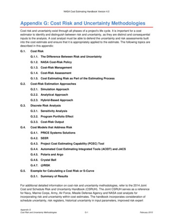
NASA Cost Estimating Handbook Version 4.0characteristics, contractor output measures, or personnel loading) to develop one or more cost estimatingrelationships (CERs). Generally, an estimator selects parametric cost estimating when only a few keypieces of data are known, such as weight and volume. The implicit assumption in parametric costestimating is that the same forces that affected cost in the past will affect cost in the future. For example,NASA cost estimates are frequently of space systems or software. The data that relate to these estimatesare weight characteristics and design complexity, respectively. The major advantage of using aparametric methodology is that the estimate can usually be conducted quickly and be easily replicated.Figure C-2 shows the steps associated with parametric cost ession)AnalysisEvaluate &Normalize DataTestRelationshipsAnalyze Data hipFigure C-2. Parametric Cost Modeling ProcessIn parametric estimating, a cost estimator will either use NASA-developed, commercial off-the-shelf(COTS), or generally accepted equations/models or create her own CERs. If the cost estimator choosesto develop her own CERs, there are several techniques to guide the estimator.To develop a parametric CER, the cost estimator must determine the drivers that most influence cost.After studying the technical baseline and analyzing the data through scatter charts and other methods,the cost estimator should verify the selected cost drivers by discussing them with engineers, scientists,and/or other technical experts. The CER can then be developed with a mathematical expression, whichcan range from a simple rule of thumb (e.g., dollars per kg) to an equation having several parameters(e.g., cost as a function of kilowatts, source lines-of-code [SLOC], and kilograms) that drive cost.Estimates created using a parametric approach are based on historical data and mathematicalexpressions relating cost as the dependent variable to selected, independent, cost-driving variables.Generally, an estimator selects parametric cost estimating when only a few key pieces of data, such asweight and volume, are known. The implicit assumption of parametric cost estimating is that the sameforces that affected cost in the past will affect cost in the future. For example, NASA cost estimates arefrequently of space systems or software. The data that relates to estimates of these are weightcharacteristics and design complexity, respectively.Appendix CCost Estimating MethodologiesC-6February 2015

NASA Cost Estimating Handbook Version 4.0The major advantage of using a parametric methodology is that the estimate can usually be conductedquickly and be easily replicated. Most estimates are developed using a variety of methods where somegeneral principles apply.Note that there are many cases when CERs can be created without the application of regressionanalysis. These CERs are typically shown as rates, factors, and ratios. Rates, factors, and ratios are oftenthe result of simple calculations (like averages) and many times do not include statistics. A rate uses a parameter to predict cost, using a multiplicative relationship. Since rate is defined to becost as a function of a parameter, the units for rate are always dollars per something. The rate mostcommonly used in cost estimating is the labor rate, expressed in dollars per hour. Other commonlyused rates are dollars per pound and dollars per gallon. A factor uses the cost of another element to estimate a new cost using a multiplier. Since a factor isdefined to be cost as a function of another cost, it is often expressed as a percentage. For example,travel costs may be estimated as 5 percent of program management costs. A ratio is a function of another parameter and is often used to estimate effort. For example, the costto build a component could be based on the industry standard of 20 hours per subcomponent.Parametric estimates established early in the acquisition process must be periodically examined toensure that they are current throughout the acquisition life cycle and that the input range of data beingestimated is applicable to the system. Such output should be shown in detail and well documented. If, forexample, a CER is improperly applied, a serious estimating error could result. Microsoft Excel and othercommercially available modeling tools are most often used for these calculations. For more information onmodels and tools, refer to Appendix E.The remainder of the parametrics section will cover how a cost estimator applies regression analysis tocreate a CER and uses analysis of variance (ANOVA) to evaluate the quality of the CER.Regression analysis is the primary method by which parametric cost estimating is enabled. Regressionis a branch of applied statistics that attempts to quantify the relationship between variables and thendescribe the accuracy of that relationship by various indicators. This definition has two parts: (1)quantifying the relationship between the variables involves using a mathematical expression, and (2)describing the accuracy of the relationship requires the computation of various statistics that indicate howwell the mathematical expression describes the relationship between the variables. This chapter coversmathematical expressions that describe the relationship between the variables using a linear expressionwith only two variables. The graphical representation of this expression is a straight line. Regressionanalysis is the technique applied in the parametric method of cost estimating. Some basic statistics textsalso refer to regression analysis as the Least Square Best Fit (LSBF) method, also known as the methodof Ordinary Least Squares (OLS).The main challenge in analyzing bivariate (two variable) and multivariate (three or more variables) data isto discover and measure the association or covariation between the variables—that is, to determine howthe variables relate to one another. When the relationship between variables is sharp and precise,ordinary mathematical methods suffice. Algebraic and trigonometric relationships have been studiedsuccessfully for centuries. When the relationship is blurred or imprecise, the preference is to usestatistical methods. We can measure whether the vagueness is so great that there is no usefulrelationship at all. If there is only a moderate amount of vagueness, we can calculate what the bestprediction would be and also qualify the prediction to take into account the imprecision of the relationship.There are two related, but distinct, aspects of the study of association between variables. The first,regression analysis, attempts to establish the nature of the relationship between variables—that is, tostudy the functional relationship between the variables and thereby provide a mechanism for predicting orAppendix CCost Estimating MethodologiesC-7February 2015

NASA Cost Estimating Handbook Version 4.0forecasting. The second, correlation analysis, has the objective of determining the degree of therelationship between variables. In the context of this appendix, we employ regression analysis to developan equation or CER.If there is a relationship between any variables, there are four possible reasons.1. The first reason has the least utility: chance. Everyone is familiar with this type of unexpected andunexplainable event. An example of a chance relationship might be a person totally unfamiliarwith the game of football winning a football pool by correctly selecting all the winning teams. Thistype of relationship between variables is totally useless since it is unquantifiable. There is no wayto predict whether or when the person would win again.2. A second reason for relationships between variables might be a relationship to a third set ofcircumstances. For instance, while the sun is shining in the United States, it is nighttime inAustralia. Neither event caused the other. The relationship between these two events is betterexplained by relating each event to another variable, the rotation of Earth with respect to the Sun.Although many relationships of this form are quantifiable, we generally desire a more directrelationship.3. The third reason for correlation is a functional relationship, one which we represent by equations.An example would be the relationship: F ma, where F force, m mass, and a accelerationdue to the force of gravity. This precise relationship seldom exists in cost estimating.4. The last reason is a causal relationship. These relationships are also represented by equations,but in this case a cause-and-effect situation is inferred between the variables. It should be notedthat a regression analysis does not prove cause and effect. Instead, a regression analysispresents what the cost estimator believes to be a logical cause-and-effect relationship. It’simportant to note that each causal relationship enables the analyst to imply that the relationshipbetween variables is consistent. Therefore, two different types of variables will arise.a. There will be unknown variables called dependent variables designated by the symbol Y.b. There will be known variables called independent variables designated by the symbol X.c. The dependent variable responds to changes in the independent variable.d. When working with CERs, the Y variable represents some sort of cost, while the X variablesrepresent various parameters of the system.As noted above in #4, regression analysis is used not to confirm causality, but rather to infer causality.In other words, no matter the statistical significance of a regression result, causality cannot be proven.For example, assume a project designing a NASA launch system wants to know its cost based uponcurrent system requirements. The cost estimator investigates how well these requirements correlate tocost. If certain system requirements (e.g., thrust) indicate a strong correlation to system cost, and theseregressions appear logical (i.e., positive correlation), then one can infer that these equations have acausal relationship—a subtle yet important distinction from proving cause and effect. Although regressionanalysis cannot confirm causality, it does explicitly provide a way to (a) measure the strength ofquantitative relationships and (b) estimate and test hypotheses regarding a model’s parameters.Prior to performing regression analysis, it is important to examine and normalize the data as follows 3:(1) Make inflation adjustments to a common base year.(2) Make learning curve adjustments to a common specified unit, e.g., Cost of First Unit (CFU).(3) Check independent variables for extrapolation.(4) Perform a scatterplot analysis.3For more details on data normalization, refer to Task 7 (Gather and Normalize Data) in section 2.2.4 of the Cost EstimatingHandbook.Appendix CCost Estimating MethodologiesC-8February 2015

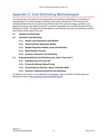
NASA Cost Estimating Handbook Version 4.0(5) Check for database homogeneity.(6) Check for multicollinearity.The first step of the actual regression analysis is to postulate what independent variable or variables (e.g.,a system’s weight, X) could have a significant effect on the dependent variable (e.g., a system’s cost, Y).This step is commonly performed by creating a scatterplot of the (X, Y) data pairs then “eyeballing” toidentify a possible trend. For a CER, the dependent variable will always be cost and each independentvariable will be a cost driver. Each cost driver should be chosen only when there is correlation between itand cost and because there are sound principles for the relationship being investigated. For example,given analysts assume that the complexity (X) of a piece of computer software drives the cost of asoftware development project (Y), the analysts can investigate their assumption by plotting historical pairsof these dependent and independent variables (Y versus X). Plotting this historical data of cost (Y) versusweight (X) produces a scatterplot as shown in Figure C-3.350–C O S TGiven weight (X) 675; cost (Y) 240300–250–240Regression CalculationY aX bY 0.355 * X 0.703Y 0.355 * 675 0.703 240200–5005506006507007508008509009501000W E I G H TFigure C-3. Scatterplot and Regression Line of Cost (Y) Versus Weight (X)The point of regression analysis is to “fit” a line to the data that will result in an equation that describesthat line, expressed by Y Y-intercept (slope) (X). In Figure C-1, we assume a positive correlation, onethat indicates that as weight increases, so does the cost associated with the weight. It is much lesscommon that a CER will be developed around a negative correlation, i.e., as the independent variableincreases in quantity, cost decreases. Whether the independent variable is complexity or weight orsomething else, there is typically a positive correlation to cost.The next step in performing regression analysis to produce a CER is to calculate the relationship betweenthe dependent (Y) and independent (X) variables. In other words, see if the data infer any reasonabledegree of cause and effect. The data are, in most cases, assumed to follow either a linear or nonlinearpattern. For the regression line in Figure C-1, the notional CER is depicted as a linear relationship of Cost A B * Weight.Appendix CCost Estimating MethodologiesC-9February 2015

NASA Cost Estimating Handbook Version 4.0As noted in the beginning of this section, the most widely used regression method is the OLS method,which can be applied for modeling both linear and nonlinear CERs (when having one independentvariable). Through the application of OLS, section C.2.1. provides details on how to model dependent andindependent variables in linear equation form, Y Y-intercept (slope) (X). OLS is used again in sectionC.2.2. to calculate nonlinear models of the form Y AXB. In order to apply OLS in section C.2.2. (on whatis thought to be a nonlinear trend), the nonlinear historical (X, Y) data is transformed using logarithms.Table C-4 serves as a reference for describing key symbols used in regression analysis. This summarytable includes not only symbols that make up a regression model but also important symbols used toassess these models.There are several other regression methods to produce nonlinear models that bypass the need totransform the historical (X, Y) data. These methods, which were developed to address limitationsassociated with OLS, include: Minimum Unbiased Percentage Error (MUPE) MethodZero Percent Bias/Minimum Percent Error (ZPB/MPE) Method (also known as ZMPE Method)Iterative Regression TechniquesSuch nonlinear regression methods are out of the scope of this handbook and, therefore, will not becovered in Appendix C. For more information on the MUPE Method, ZMPE Method, and IterativeRegression Techniques, refer to the “Regression Methods” section of Appendix A of the 2013 Joint Costand Schedule Risk and Uncertainty Handbook (CSRUH) at https://www.ncca.navy.mil/tools/tools.cfm.The remainder of Section C.2. covers the following steps in performing regression analysis and selectingthe best CER:(1) Review the literature and scatterplots to postulate cost drivers of the dependent variable.(2) Select the independent variables(s) for each CER.(3) Specify each model’s functional form (e.g., linear, nonlinear).(4) Apply regression methods to produce each CER.(5) Perform significance tests (i.e., t-test, F-test) and residual analyses.(6) Test for multicollinearity (if multiple regression).(7) See if equation causality seems logical (e.g., does the sign of slope coefficient make sense?).(8) For remaining equations, down-select to the one with highest R2 and/or lowest SE.(9) Collect additional data and repeat steps 1–8 (if needed).(10) Document the results.These steps begin with how to produce and assess a simple linear regression (SLR) model.Appendix CCost Estimating MethodologiesC-10February 2015

NASA Cost Estimating Handbook Version 4.0Table C-4. Summary of Key Symbols in Regression AnalysisSymbolDescriptionDefinitionX, YData ObservationsY dependent variableX independent variableX ,YAverage or MeanXYX i 's mean of actual Yi 's. mean of actualEvaluationCheck and correct any errors,especially outliers in the data. If dataquality is poor, it may be necessary toopt for an analysis method other thanregression.Helpful to describe the central tendencyof the data being evaluated Derived using SLR, YiCalculated YYiYiis the predictedXi ,and will differ from Yi whenever Yior “fitted” value associated with dependent variabledoes not lie on the regression line.Estimated Coefficientof Each IndependentVariable (i.e., eachestimated regressionparameter)Value of y-intercept, eachslope in a linear equation,and/or each exponent in anonlinear equationIf t-stats are below threshold or valuesseem illogical, re-specify the model(e.g., with other independent variablesand/or another functional form).eiError or “Residual”Difference between anactual Y (Yi) and itsrespective predicted Y (Y)Check for transcription errors. Takeappropriate corrective action.R2Coefficient ofDeterminationMeasures degree ofoverall fit of the model tothe dataThe closer R2 is to 100 percent, thebetter the fit.b i or BiR 2aR2Adjusted forDegrees of FreedomR2 formula is adjusted toaccount for contribution ofone or more additionalexplanatory variables.SSRSSESum of Squared TotalSum of SquaredRegression(Explained Error)Sum of SquaredErrors(Unexplained Error)SST SSR Σvariable is irrelevant is if the value(Yi – Y)2R 2agoes down when the explanatoryvariable is added to the equation.Used to compute R2 andnSSTOne indication that an explanatoryR 2a . Thei 1higher the SST, the more disperse theactual Y-data is from the mean of Y.nUsed to compute R2 andΣ(Yi – Y)2R 2a . Thei 1higher the SSR, the more “different” theregression line is from the mean of Y.nUsed to compute R2 and i )2SSE Σ (Yi – Yi 1R 2a . Thehigher the SSE, the more disperse thepredicted Y-data is from a

Power 2.3 KW 3.4 KW Solar Array Cost 10M ? Assuming a linear relationship between power and cost, and assuming also that power is a cost driver of solar array cost, the single-point analogy calculation can