Transcription
Statistical Methods in Credit Risk ModelingbyAijun ZhangA dissertation submitted in partial fulfillmentof the requirements for the degree ofDoctor of Philosophy(Statistics)in The University of Michigan2009Doctoral Committee:Professor Vijayan N. Nair, Co-ChairAgus Sudjianto, Co-Chair, Bank of AmericaProfessor Tailen HsingAssociate Professor Jionghua JinAssociate Professor Ji Zhu
cAijun Zhang2009All Rights Reserved
To my elementary school, high school and university teachersii
ACKNOWLEDGEMENTSFirst of all, I would express my gratitude to my advisor Prof. Vijay Nair for guidingme during the entire PhD research. I appreciate his inspiration, encouragement andprotection through these valuable years at the University of Michigan. I am thankfulto Julian Faraway for his encouragement during the first years of my PhD journey. Iwould also like to thank Ji Zhu, Judy Jin and Tailen Hsing for serving on my doctoralcommittee and helpful discussions on this thesis and other research works.I am grateful to Dr. Agus Sudjianto, my co-advisor from Bank of America, forgiving me the opportunity to work with him during the summers of 2006 and 2007and for offering me a full-time position. I appreciate his guidance, active supportand his many illuminating ideas. I would also like to thank Tony Nobili, Mike Bonn,Ruilong He, Shelly Ennis, Xuejun Zhou, Arun Pinto, and others I first met in 2006at the Bank. They all persuaded me to jump into the area of credit risk research; Idid it a year later and finally came up with this thesis within two more years.I would extend my acknowledgement to Prof. Kai-Tai Fang for his consistentencouragement ever since I graduated from his class in Hong Kong 5 years ago.This thesis is impossible without the love and remote support of my parents inChina. To them, I am most indebted.iii
TABLE OF CONTENTSDEDICATION . . . . . . . . . . . . . . . . . . . . . . . . . . . . . . . . . .iiACKNOWLEDGEMENTS . . . . . . . . . . . . . . . . . . . . . . . . . .iiiLIST OF FIGURES . . . . . . . . . . . . . . . . . . . . . . . . . . . . . . .viLIST OF TABLES . . . . . . . . . . . . . . . . . . . . . . . . . . . . . . . .ixABSTRACT . . . . . . . . . . . . . . . . . . . . . . . . . . . . . . . . . . .xCHAPTERI. An Introduction to Credit Risk Modeling . . . . . . . . . . . .1.1.2256691112131518II. Adaptive Smoothing Spline . . . . . . . . . . . . . . . . . . . . .241.21.31.42.12.22.32.4Two Worlds of Credit Risk . . . . . . . .1.1.1 Credit Spread Puzzle . . . . . .1.1.2 Actual Defaults . . . . . . . . .Credit Risk Models . . . . . . . . . . . .1.2.1 Structural Approach . . . . . .1.2.2 Intensity-based Approach . . . .Survival Models . . . . . . . . . . . . . .1.3.1 Parametrizing Default Intensity1.3.2 Incorporating Covariates . . . .1.3.3 Correlating Credit Defaults . . .Scope of the Thesis . . . . . . . . . . . .Introduction . . . . . . . . . . . . .AdaSS: Adaptive Smoothing Spline .2.2.1 Reproducing Kernels . . .2.2.2 Local Penalty Adaptation .AdaSS Properties . . . . . . . . . .Experimental Results . . . . . . . .iv.1.242830323638
2.52.6Summary . . . . . . . . . . . . . . . . . . . . . . . . . . . . .Technical Proofs . . . . . . . . . . . . . . . . . . . . . . . . .4546III. Vintage Data Analysis . . . . . . . . . . . . . . . . . . . . . . . .483.13.23.3.485158586065676869737478808286IV. Dual-time Survival Analysis . . . . . . . . . . . . . . . . . . . . .883.43.53.63.74.14.24.34.44.54.64.7Introduction . . . . . . . . . . . . . . . . . .MEV Decomposition Framework . . . . . . .Gaussian Process Models . . . . . . . . . . .3.3.1 Covariance Kernels . . . . . . . . .3.3.2 Kriging, Spline and Kernel Methods3.3.3 MEV Backfitting Algorithm . . . .Semiparametric Regression . . . . . . . . . .3.4.1 Single Segment . . . . . . . . . . .3.4.2 Multiple Segments . . . . . . . . . .Applications in Credit Risk Modeling . . . .3.5.1 Simulation Study . . . . . . . . . .3.5.2 Corporate Default Rates . . . . . .3.5.3 Retail Loan Loss Rates . . . . . . .Discussion . . . . . . . . . . . . . . . . . . .Technical Proofs . . . . . . . . . . . . . . . .Introduction . . . . . . . . . . . . . . . . . .Nonparametric Methods . . . . . . . . . . . .4.2.1 Empirical Hazards . . . . . . . . . .4.2.2 DtBreslow Estimator . . . . . . . .4.2.3 MEV Decomposition . . . . . . . .Structural Models . . . . . . . . . . . . . . .4.3.1 First-passage-time Parameterization4.3.2 Incorporation of Covariate Effects .Dual-time Cox Regression . . . . . . . . . . .4.4.1 Dual-time Cox Models . . . . . . .4.4.2 Partial Likelihood Estimation . . .4.4.3 Frailty-type Vintage Effects . . . . .Applications in Retail Credit Risk Modeling .4.5.1 Credit Card Portfolios . . . . . . .4.5.2 Mortgage Competing Risks . . . . .Summary . . . . . . . . . . . . . . . . . . . .Supplementary Materials . . . . . . . . . . LIOGRAPHY . . . . . . . . . . . . . . . . . . . . . . . . . . . . . . . . 137v
LIST OF FIGURESFigure1.1Moody’s-rated corporate default rates, bond spreads and NBERdated recessions. Data sources: a) Moody’s Baa & Aaa corporate bond yields 19);b) Moody’s Special Comment on Corporate Default and RecoveryRates, 1920-2008 (http://www.moodys.com/); c) NBER-dated recessions (http://www.nber.org/cycles/). . . . . . . . . . . . . . . . . . .41.2Simulated drifted Wiener process, first-passage-time and hazard rate.81.3Illustration of retail credit portfolios and vintage diagram. . . . . .191.4Moody’s speculative-grade default rates for annual cohorts 1970-2008:projection views in lifetime, calendar and vintage origination time. .21A road map of thesis developments of statistical methods in creditrisk modeling. . . . . . . . . . . . . . . . . . . . . . . . . . . . . . .22Heterogeneous smooth functions: (1) Doppler function simulated withnoise, (2) HeaviSine function simulated with noise, (3) MotorcycleAccident experimental data, and (4) Credit-Risk tweaked sample. . .26OrdSS function estimate and its 2nd-order derivative (upon standardization): scaled signal from f (t) sin(ωt) (upper panel) andf (t) sin(ωt4 ) (lower panel), ω 10π, n 100 and snr 7. Thesin(ωt4 ) signal resembles the Doppler function in Figure 2.1; bothhave time-varying frequency. . . . . . . . . . . . . . . . . . . . . . .34OrdSS curve fitting with m 2 (shown by solid lines). The dashedlines represent 95% confidence intervals. In the credit-risk case, thelog loss rates are considered as the responses, and the time-dependentweights are specified proportional to the number of replicates. . . .391.52.12.22.3vi
2.4Simulation study of Doppler and HeaviSine functions: OrdSS (blue),AdaSS (red) and the heterogeneous truth (light background). . . . .402.5Non-stationary OrdSS and AdaSS for Motorcycle-Accident Data. . .422.6OrdSS, non-stationary OrdSS and AdaSS: performance in comparison. 422.7AdaSS estimate of maturation curve for Credit-Risk sample: piecewiseconstant ρ 1 (t) (upper panel) and piecewise-linear ρ 1 (t) (lower panel). 443.1Vintage diagram upon truncation and exemplified prototypes. . . .503.2Synthetic vintage data analysis: (top) underlying true marginal effects; (2nd) simulation with noise; (3nd) MEV Backfitting algorithmupon convergence; (bottom) Estimation compared to the underlyingtruth. . . . . . . . . . . . . . . . . . . . . . . . . . . . . . . . . . .76Synthetic vintage data analysis: (top) projection views of fitted values; (bottom) data smoothing on vintage diagram. . . . . . . . . . .77Results of MEV Backfitting algorithm upon convergence (right panel)based on the squared exponential kernels. Shown in the left panel isthe GCV selection of smoothing and structural parameters. . . . . .793.5MEV fitted values: Moody’s-rated Corporate Default Rates . . . . .793.6Vintage data analysis of retail loan loss rates: (top) projection viewsof emprical loss rates in lifetime m, calendar t and vintage originationtime v; (bottom) MEV decomposition effects fˆ(m), ĝ(t) and ĥ(v) (atlog scale). . . . . . . . . . . . . . . . . . . . . . . . . . . . . . . . .823.33.44.1Dual-time-to-default: (left) Lexis diagram of sub-sampled simulations; (right) empirical hazard rates in either lifetime or calendar time. 904.2DtBreslow estimator vs one-way nonparametric estimator using thedata of (top) both pre-2005 and post-2005 vintages; (middle) pre2005 vintages only; (bottom) post-2005 vintages only. . . . . . . . .984.3MEV modeling of empirical hazard rates, based on the dual-time-todefault data of (top) both pre-2005 and post-2005 vintages; (middle)pre-2005 vintages only; (bottom) post-2005 vintages only. . . . . . . 1014.4Nonparametric analysis of credit card risk: (top) one-way empiricalhazards, (middle) DtBrewlow estimation, (bottom) MEV decomposition. . . . . . . . . . . . . . . . . . . . . . . . . . . . . . . . . . . 121vii
4.5MEV decomposition of credit card risk for low, medium and highFICO buckets: Segment 1 (top panel); Segment 2 (bottom panel). . 1234.6Home prices and unemployment rate of California state: 2000-2008.4.7MEV decomposition of mortgage hazards: default vs. prepayment . 1254.8Split time-varying covariates into little time segments, illustrated. . 133viii125
LIST OF TABLESTable1.1Moody’s speculative-grade default rates. Data source: Moody’s special comment (release: February 2009) on corporate default and recovery rates, 1920-2008 (http://www.moodys.com/) and author’s calculations. . . . . . . . . . . . . . . . . . . . . . . . . . . . . . . . . .232.1AdaSS parameters in Doppler and HeaviSine simulation study. . . . .413.1Synthetic vintage data analysis: MEV modeling exercise with GCVselected structural and smoothing parameters. . . . . . . . . . . . .774.1Illustrative data format of pooled credit card loans . . . . . . . . . . 1204.2Loan-level covariates considered in mortgage credit risk modeling,where NoteRate could be dynamic and others are static upon origination. . . . . . . . . . . . . . . . . . . . . . . . . . . . . . . . . . . 1284.3Maximum partial likelihood estimation of mortgage covariate effectsin dual-time Cox regression models. . . . . . . . . . . . . . . . . . . 128ix
ABSTRACTThis research deals with some statistical modeling problems that are motivatedby credit risk analysis. Credit risk modeling has been the subject of considerableresearch interest in finance and has recently drawn the attention of statistical researchers. In the first chapter, we provide an up-to-date review of credit risk modelsand demonstrate their close connection to survival analysis.The first statistical problem considered is the development of adaptive smoothing spline (AdaSS) for heterogeneously smooth function estimation. Two challengingissues that arise in this context are evaluation of reproducing kernel and determination of local penalty, for which we derive an explicit solution based on piecewisetype of local adaptation. Our nonparametric AdaSS technique is capable of fitting adiverse set of ‘smooth’ functions including possible jumps, and it plays a key role insubsequent work in the thesis.The second topic is the development of dual-time analytics for observations involving both lifetime and calendar timescale. It includes “vintage data analysis”(VDA) for continuous type of responses in the third chapter, and “dual-time survivalanalysis” (DtSA) in the fourth chapter. We propose a maturation-exogenous-vintage(MEV) decomposition strategy in order to understand the risk determinants in termsof self-maturation in lifetime, exogenous influence by macroeconomic conditions, andheterogeneity induced from vintage originations. The intrinsic identification problemis discussed for both VDA and DtSA. Specifically, we consider VDA under Gaussian process models, provide an efficient MEV backfitting algorithm and assess itsperformance with both simulation and real examples.x
DtSA on Lexis diagram is of particular importance in credit risk modeling wherethe default events could be triggered by both endogenous and exogenous hazards.We consider nonparametric estimators, first-passage-time parameterization and semiparametric Cox regression. These developments extend the family of models for bothcredit risk modeling and survival analysis. We demonstrate the application of DtSAto credit card and mortgage risk analysis in retail banking, and shed some light onunderstanding the ongoing credit crisis.xi
CHAPTER IAn Introduction to Credit Risk ModelingCredit risk is a critical area in banking and is of concern to a variety of stakeholders: institutions, consumers and regulators. It has been the subject of considerableresearch interest in banking and finance communities, and has recently drawn theattention of statistical researchers. By Wikipedia’s definition,“Credit risk is the risk of loss due to a debtor’s non-payment of a loanor other line of credit.” (Wikipedia.org, as of March 2009)Central to credit risk is the default event, which occurs if the debtor is unable tomeet its legal obligation according to the debt contract. The examples of defaultevent include the bond default, the corporate bankruptcy, the credit card chargeoff, and the mortgage foreclosure. Other forms of credit risk include the repaymentdelinquency in retail loans, the loss severity upon the default event, as well as theunexpected change of credit rating.An enormous literature in credit risk has been fostered by both academics infinance and practitioners in industry. There are two parallel worlds based upon asimple dichotomous rule of data availability: (a) the direct measurements of creditperformance and (b) the prices observed from credit market. The data availabilityleads to two streams of credit risk modeling that have key distinctions.1
1.1Two Worlds of Credit RiskThe two worlds of credit risk can be simply characterized by the types of defaultprobability, one being actual and the other being implied. The former correspondsto the direct observations of defaults, also known as the physical default probabilityin finance. The latter refers to the risk-neutral default probability implied from thecredit market data, e.g. corporate bond yields.The academic literature of corporate credit risk has been inclined to the study ofthe implied defaults, which is yet a puzzling world.1.1.1Credit Spread PuzzleThe credit spread of a defaultable corporate bond is its excess yield over thedefault-free Treasury bond of the same time to maturity. Consider a zero-couponcorporate bond with unit face value and maturity date T . The yield-to-maturity att T is defined byY (t, T ) log B(t, T )T t(1.1)where B(t, T ) is the bond price of the form Z T(r(s) λ(s))ds ,B(t, T ) E exp (1.2)tgiven the independent term structures of the interest rate r(·) and the default rateλ(·). Setting λ(t) 0 gives the benchmark price B0 (t, T ) and the yield Y0 (t, T ) ofTreasury bond. Then, the credit spread can be calculated asSpread(t, T ) Y (t, T ) Y0 (t, T ) log(B(t, T )/B0 (t, T ))log(1 q(t, T )) T tT t(1.3) RT where q(t, T ) E e t λ(t)ds is the conditional default probability P[τ T τ t] andτ denotes the time-to-default, to be detailed in the next section.2
The credit spread is supposed to co-move with the default rate. For illustration,Figure 1.1 (top panel) plots the Moody’s-rated corporate default rates and BaaAaa bond spreads ranging from 1920-2008. The shaded backgrounds correspond toNBER’s latest announcement of recession dates. Most spikes of the default rates andthe credit spreads coincide with the recessions, but it is clear that the movements oftwo time series differ in both level and change. Such a lack of match is the so-calledcredit spread puzzle in the latest literature of corporate finance; the actual defaultrates could be successfully implied from the market data of credit spreads by none ofthe existing structural credit risk models.The default rates implied from credit spreads mostly overestimate the expecteddefault rates. One factor that helps explain the gap is the liquidity risk – a security cannot be traded quickly enough in the market to prevent the loss. Figure 1.1(bottom panel) plots, in fine resolution, the Moody’s speculative-grade default ratesversus the high-yield credit spreads: 1994-2008. It illustrates the phenomenon wherethe spread changed in response to liquidity-risk events, while the default rates did notreact significantly until quarters later; see the liquidity crises triggered in 1998 (Russian/LTCM shock) and 2007 (Subprime Mortgage meltdown). Besides the liquidityrisk, there exist other known (e.g. tax treatments of corporate bonds vs. governmentbonds) and unknown factors that make incomplete the implied world of credit risk.As of today, we lack a thorough understanding of the credit spread puzzle; see e.g.Chen, Lesmond and Wei (2007) and references therein.The shaky foundation of the default risk implied from market credit spreads without looking at the historical defaults leads to further questions about the creditderivatives, e.g. Credit Default Swap (CDS) and Collateralized Debt Obligation(CDO). The 2007-08 collapse of credit market in Wall Street is partly due to overcomplication in “innovating” such complex financial instruments on the one hand,and over-simplification in quantifying their embedded risks on the other.3
Figure 1.1: Moody’s-rated corporate default rates, bond spreads and NBERdated recessions.Data sources: a) Moody’s Baa & Aaa corporate bond yields 19);b) Moody’s Special Comment on Corporate Default and RecoveryRates, 1920-2008 (http://www.moodys.com/); c) NBER-dated recessions(http://www.nber.org/cycles/).4
1.1.2Actual DefaultsThe other world of credit risk is the study of default probability bottom up fromthe actual credit performance. It includes the popular industry practices ofa) credit rating in corporate finance, by e.g. the three major U.S. rating agencies:Moody’s, Standard & Poor’s, and Fitch.b) credit scoring in consumer lending, by e.g. the three major U.S. credit bureaus:Equifax, Experian and TransUnion.Both credit ratings and scores represent the creditworthiness of individual corporations and consumers. The final evaluations are based on statistical models of theexpected default probability, as well as judgement by rating/scoring specialists. Letus describe very briefly some rating and scoring basics related to the thesis.The letters Aaa and Baa in Figure 1.1 are examples of Moody’s rating system,which use Aaa, Aa, A, Baa, Ba, B, Caa, Ca, C to represent the likelihood of defaultfrom the lowest to the highest. The speculative grade in Figure 1.1 refers to Ba andthe worse ratings. The speculative-grade corporate bonds are sometimes said to behigh-yield or junk.FICO, developed by Fair Isaac Corporation, is the best-known consumer creditscore and it is the most widely used by U.S. banks and other credit card or mortgagelenders. It ranges from 300 (very poor) to 850 (best), and intends to represent thecreditworthiness of a borrower such that he or she will repay the debt. For the sameborrower, the three major U.S. credit bureaus often report inconsistent FICO scoresbased on their own proprietary models.Compared to either the industry practices mentioned above or the academics ofthe implied default probability, the academic literature based on the actual defaultsis much smaller, which we believe is largely due to the limited access for an academicresearcher to the proprietary internal data of historical defaults. A few academic5
works will be reviewed later in Section 1.3. In this thesis, we make an attemptto develop statistical methods based on the actual credit performance data. Fordemonstration, we shall use the synthetic or tweaked samples of retail credit portfolios,as well as the public release of corporate default rates by Moody’s.1.2Credit Risk ModelsThis section reviews the finance literature of credit risk models, including bothstructural and intensity-based approaches. Our focus is placed on the probability ofdefault and the hazard rate of time-to-default.1.2.1Structural ApproachIn credit risk modeling, structural approach is also known as the firm-value approach since a firm’s inability to meet the contractual debt is assumed to be determined by its asset value. It was inspired by the 1970s Black-Scholes-Merton methodology for financial option pricing. Two classic structural models are the Merton model(Merton, 1974) and the first-passage-time model (Black and Cox, 1976).The Merton model assumes that the default event occurs at the maturity dateof debt if the asset value is less than the debt level. Let D be the debt level withmaturity date T , and let V (t) be the latent asset value following a geometric BrownianmotiondV (t) µV (t)dt σV (t)dW (t),(1.4)with drift µ, volatility σ and the standard Wiener process W (t). Recall that EW (t) 0, EW (t)W (s) min(t, s). Given the initial asset value V (0) D, by Itó’s lemma, V (t)1 2 1 2 2 expµ σ t σWt Lognormal µ σ t, σ t ,V (0)22from which one may evaluate the default probability P(V (T ) D).6(1.5)
The notion of distance-to-default facilitates the computation of conditional defaultprobability. Given the sample path of asset values up to t, one may first estimate theunknown parameters in (1.4) by maximum likelihood method. According to Duffieand Singleton (2003), let us define the distance-to-default X(t) by the number ofstandard deviations such that log Vt exceeds log D, i.e.X(t) (log V (t) log D)/σ.(1.6)Clearly, X(t) is a drifted Wiener process of the formX(t) c bt W (t),with b µ σ 2 /2σand c log V (0) log D.σt 0(1.7)Then, it is easy to verify that the conditionalprobability of default at maturity date T is P(V (T ) D V (t) D) P(X(T ) 0 X(t) 0) ΦX(t) b(T t) T t ,(1.8)where Φ(·) is the cumulative normal distribution function.The first-passage-time model by Black and Cox (1976) extends the Merton modelso that the default event could occur as soon as the asset value reaches a pre-specifieddebt barrier. Figure 1.2 (left panel) illustrates the first-passage-time of a driftedWiener process by simulation, where we set the parameters b 0.02 and c 8 (s.t.a constant debt barrier). The key difference of Merton model and Black-Cox modellies in the green path (the middle realization viewed at T ), which is treated as defaultin one model but not the other.By (1.7) and (1.8), V (t) hits the debt barrier once the distance-to-default processX(t) hits zero. Given the initial distance-to-default c X(0) 0, consider the7
Figure 1.2: Simulated drifted Wiener process, first-passage-time and hazard rate.first-passage-timeτ inf{t 0 : X(t) 0},(1.9)where inf as usual. It is well known that τ follows the inverse Gaussiandistribution (Schrödinger, 1915; Tweedie, 1957; Chhikara and Folks, 1989) with thedensity (c bt)2c 3/2exp f (t) t,2t2πt 0.(1.10)See also other types of parametrization in Marshall and Olkin (2007; §13). Thesurvival function S(t) is defined by P(τ t) for any t 0 and is given by S(t) Φc bt t 2bc e Φ c bt t .(1.11)The hazard rate, or the conditional default rate, is defined by the instantaneousrate of default conditional on the survivorship,1f (t)P(t τ t t τ t) . t 0 tS(t)λ(t) lim(1.12)Using the inverse Gaussian density and survival functions, we obtain the form of the8
first-passage-time hazard rate: (c bt)2 exp 2t2πt3 , λ(t; c, b) c btc bt 2bc eΦΦttcc 0.(1.13)This is one of the most important forms of hazard function in structural approachto credit risk modeling. Figure 1.2 (right panel) plots λ(t; c, b) for b 0.02 andc 4, 6, 8, 10, 12, which resemble the default rates from low to high credit qualitiesin terms of credit ratings or FICO scores. Both the trend parameter b and the initialdistance-to-default parameter c provide insights to understanding the shape of thehazard rate; see the details in Chapter IV or Aalen, Borgan and Gjessing (2008; §10).Modern developments of structural models based on Merton and Black-Cox models can be referred to Bielecki and Rutkowski (2004; §3). Later in Chapter IV, wewill discuss the dual-time extension of first-passage-time parameterization with bothendogenous and exogenous hazards, as well as non-constant default barrier and incomplete information about structural parameters.1.2.2Intensity-based ApproachThe intensity-based approach is also called the reduced-form approach, proposedindependently by Jarrow and Turnbull (1995) and Madan and Unal (1998). Manyfollow-up papers can be found in Lando (2004), Bielecki and Rutkowski (2004) andreferences therein. Unlike the structural approach that assumes the default to becompletely determined by the asset value subject to a barrier, the default event in thereduced-form approach is governed by an externally specified intensity process thatmay or may not be related to the asset value. The default is treated as an unexpectedevent that comes ‘by surprise’. This is a practically appealing feature, since in thereal world the default event (e.g. Year 2001 bankruptcy of Enron Corporation) is9
often all of a sudden happening without announcement.The default intensity corresponds to the hazard rate λ(t) f (t)/S(t) defined in(1.12) and it has roots in statistical reliability and survival analysis of time-to-failure.When S(t) is absolutely continuous with f (t) d(1 S(t))/dt, we have that dS(t)d[log S(t)]λ(t) ,S(t)dtdt Z tλ(s)ds ,S(t) exp t 0.0In survival analysis, λ(t) is usually assumed to be a deterministic function in time.In credit risk modeling, λ(t) is often treated as stochastic. Thus, the default timeτ is doubly stochastic. Note that Lando (1998) adopted the term “doubly stochasticPoisson process” (or, Cox process) that refers to a counting process with possiblyrecurrent events. What matters in modeling defaults is only the first jump of thecounting process, in which case the default intensity is equivalent to the hazard rate.In finance, the intensity-based models are mostly the term-structure models borrowed from the literature of interest-rate modeling. Below is an incomplete list:Vasicek:Cox-Ingersoll-Roll:Affine jump:dλ(t) κ(θ λ(t))dt σdWtpdλ(t) κ(θ λ(t))dt σ λ(t)dWt(1.14)dλ(t) µ(λ(t))dt σ(λ(t))dWt dJtwith reference to Vasicek (1977), Cox, Ingersoll and Roll (1985) and Duffie, Pan andSingleton (2000). The last model involves a pure-jump process Jt , and it covers boththe mean-reverting Vasicek and CIR models by setting µ(λ(t)) κ(θ λ(t)) andpσ(λ(t)) σ02 σ12 λ(t).The term-structure models provide straightforward ways to simulate the futuredefault intensity for the purpose of predicting the conditional default probability.However, they are ad hoc models lacking fundamental interpretation of the defaultevent. The choices (1.14) are popular because they could yield closed-form pricing10
formulas for (1.2), while the real-world default intensities deserve more flexible andmeaningful forms. For instance, the intensity models in (1.14) cannot be used tomodel the endogenous shapes of first-passage-time hazards illustrated in Figure 1.2.The dependence of default intensity on state variables z(t) (e.g. macroeconomiccovariates) is usually treated through a multivariate term-structure model for thejoint of (λ(t), z(t)). This approach essentially presumes a linear dependence in thediffusion components, e.g. by correlated Wiener processes. In practice, the effect ofa state variable on the default intensity can be non-linear in many other ways.The intensity-based approach also includes the duration models for econometricanalysis of actual historical defaults. They correspond to the classical survival analysisin statistics, which opens another door for approaching credit risk.1.3Survival ModelsCredit risk modeling in finance is closely related to survival analysis in statistics, including both the first-passage-time structural models and the duration typeof intensity-based models. In a rough sense, default risk models based on the actualcredit performance data exclusively belong to survival analysis, since the latter bydefinition is the analysis of time-to-failure data. Here, the failure refers to the defaultevent in either corporate or retail risk exposures; see e.g. Duffie, Saita and Wang(2007) and Deng, Quigley and Van Order (2000).We find that the survival models have at least four-fold advantages in approachto credit risk modeling:1. flexibility in parametrizing the default intensity,2. flexibility in incorporating various types of covariates,3. effectiveness in modeling the credit portfolios, and11
4. being straightforward to enrich and extend the family of credit risk models.The following materials are organized in a way to make these points one by one.1.3.1Parametrizing Default IntensityIn survival analysis, there are a rich set of lifetime distributions for parametrizingthe default intensity (i.e. hazard rate) λ(t), c:λ(t) αλ(t) αtβ 1(1.15)1 φ(log t/α)tα Φ( log t/α)(β/α)(t/α)β 1λ(t) ,1 (t/α)βλ(t) α, β 0where φ(x) Φ0 (x) is the density function of normal distribution. Another exampleis the inverse Gaussian type of hazard rate function in (1.13). More examples ofparametric models can be found in Lawless (2003) and Marshall and
Statistical Methods in Credit Risk Modeling by Aijun Zhang A dissertation submitted in partial ful llment of the requirements for the degree of Doctor of Philosophy (Statistics) in The University of Michigan 2009 Doctoral Committee: Professor Vijayan N. Nair, Co-Chair Agus Su