Transcription
Basic Statistical and Modeling Procedures Using SASOne-Sample TestsThe statistical procedures illustrated in this handout use two datasets. The first, Pulse, hasinformation collected in a classroom setting, where students were asked to take their pulse twotimes. Half the class was asked to run in place between the two readings and the other group wasasked to stay seated between the two readings. The raw data for this study are contained in a filecalled pulse.csv. The other dataset we use is a dataset called Employee.sas7bdat. It is a SASdataset that contains information about salaries in a mythical company.Read in the pulse data and create a temporary SAS dataset for the examples:data pulse;infile "pulse.csv" firstobs 2 delimiter "," missover;input pulse1 pulse2 ran smokes sex height weight activity;label pulse1 "Resting pulse, rate per minute"pulse2 "Second pulse, rate per minute";run;Create and assign formats to variables:proc format;value sexfmt 1 "Male" 2 "Female";value yesnofmt 1 "Yes" 2 "No";value actfmt 1 "Low" 2 "Medium" 3 "High";run;proc print data pulse (obs 25) label;format sex sexfmt. ran smokes yesnofmt. activity actfmt.;run;Descriptive Statistics:proc means data pulse;run;The MEANS ProcedureVariable LabelNMeanStd ----------------pulse1Resting pulse, rate per minute econd pulse, rate per ------------------1
Binomial Confidence Intervals and Tests for Binary Variables:If you have a categorical variable with only two levels, you can use the binomial option torequest a 95% confidence interval for the proportion in the first level of the variable. In thePULSE data set, SMOKES 1 indicates those who were smokers, and SMOKES 2 indicatesnon-smokers. Use the (p ) option to specify the null hypothesis proportion that you wish to testfor the first level of the variable. In the commands below, we test hypotheses for the proportionof SMOKES 1 (i.e., proportion of smokers) in the population. By default SAS produces anasymptotic test of the null hypothesis:H0: proportion of smokers 0.25HA: proportion of smokers 0.25proc freq data pulse;tables smokes / binomial(p 9.5792100.00Binomial Proportionfor smokes E0.048095% Lower Conf Limit0.210395% Upper Conf Limit0.3984Exact Conf Limits95% Lower Conf Limit95% Upper Conf Limit0.21270.4090Test of H0: Proportion 0.25ASE under H0ZOne-sided Pr ZTwo-sided Pr Z 0.04511.20390.11430.2286Sample Size 92If you wish to obtain an exact binomial test of the null hypothesis, use the exact statement. If youinclude the mc option for large datasets, you will get a Monte Carlo p-value.proc freq data pulse;tables smokes / binomial(p .25);exact binomial / mc;run;2
This results in an exact test of the null hypothesis, in addition to the default asymptotic test, theexact test results for both a one-sided and two-sided alternative hypothesis are shown.Binomial Proportion for smokes 1----------------------------------Proportion (P)0.3043ASE0.048095% Lower Conf Limit0.210395% Upper Conf Limit0.3984Exact Conf Limits95% Lower Conf Limit95% Upper Conf Limit0.21270.4090Test of H0: Proportion 0.25ASE under H0ZOne-sided Pr ZTwo-sided Pr Z 0.04511.20390.11430.2286Exact TestOne-sided Pr PTwo-sided 2 * One-sidedSample Size 920.13990.2797Chi-square Goodness of Fit Tests for Categorical Variables:Use the chisq option in the tables statement to get a chi-square goodness of fit test, which can beused for categorical variables with two or more levels. By default SAS assumes that you wish totest the null hypothesis that the proportion of cases is equal in all categories. In the variableACTIVITY, a value of 1 indicates a low level of activity, a value of 2 is a medium level ofactivity, and a value of 3 indicates a high level of activity.proc freq data pulse;tables activity / .8726166.307177.1732122.8392100.00Chi-Square Testfor Equal 2Pr ChiSq .0001Sample Size 923
If you wish to specify your own proportions, use the testp option in the tables statement. Thisoption allows you to specify any proportions that you wish to test for each level of the variable inthe tables statement, as long as the sum of the proportions equals 1.0. In the example below wetest the null hypothesis:H0: P1 0.20, P2 .50, P3 .30proc freq data pulse;tables activity /chisq testp ( .20 , .50, .30 );run;The FREQ 32122.8330.0092100.00Chi-Square Testfor Specified 43DF2Pr ChiSq0.0058Sample Size 92You may also specify percentages to test, rather than proportions, as long as they add up to 100percent:proc freq data pulse;tables activity /chisq testp ( 20 , 50, 30 );run;One-Sample test for a continuous variable:You can use Proc Univariate to carry out a one-sample t-test to test the population mean againstany null hypothesis value you specify by using mu0 option. The default, if no value of mu0 isspecified is that mu0 0. In the commands below, we test:H0: 0 72HA: 0 72Note that SAS also provides the non-parametric Sign test and Wilcoxon signed rank test.4
proc univariate data pulse mu0 72;var pulse1;histogram / normal (mu est sigma est);qqplot /normal (mu est sigma est);run;Selected output from Proc Univariate:Proc UnivariateTests for Location: Mu0 72Test-Statistic-----p Value-----Student's tt 0.757635Pr t 0.4506SignM-3Pr M 0.5900Signed RankS96.5Pr S 060rminu550te40052606876Re s t i n gpul s e,84r at eper92- 3100- 2- 10No r ma lmi n u t e123Qu a n t i l e sEquivalently, we can carry out a one-sample t-test in Proc Ttest by specifying the H0 option.:proc ttest data pulse H0 72 ;var 1(Resting pulse, rate per minuteStd Dev11.0087Std Err1.147795% CL Mean70.5897 75.1494DF91Minimum48.0000Std Dev11.0087t Value0.76Maximum100.095% CL Std Dev9.6155 12.8779Pr t 0.4506Paired Samples t-test:If you wish to compare the means of two variables that are paired (i.e. correlated), you can use apaired sample t-test for continuous variables. To do this use Proc ttest with a paired statement,to get a paired samples t-test:proc ttest data pulse;paired pulse2*pulse1;run;5
Differencepulse2 - pulse1N92Lower CLMean4.3406The TTEST ProcedureStatisticsUpper CL Lower CLMeanMeanStd Dev7.13049.920311.766T-TestsDFt Value915.08Differencepulse2 - pulse1Std Dev13.471Upper CLStd Dev15.759Std Err1.4045Pr t .0001The paired t-test can be carried out for each level of RAN. The commands and results of thesecommands are shown below:proc sort data pulse;by ran;run;proc ttest data pulse;paired pulse2*pulse1;by ran;run;---------------------------------------- ran 1 --------------------------------------------The TTEST ProcedureStatisticsDifferencepulse2 - pulse1N35Lower CLMean13.745Upper CLMean24.084Mean18.914Differencepulse2 - pulse1T-TestsDF34Lower CLStd Dev12.173t Value7.44Std Dev15.05Upper CLStd Dev19.718Std Err2.5439Pr t .0001--------------------------------------------- ran 2 --------------------------------------------The TTEST ProcedureStatisticsDifferencepulse2 - pulse1N57Lower CLMean-1.209Mean-0.105Differencepulse2 - pulse1Upper CLMean0.9987Lower CLStd Dev3.5126T-TestsDFt Value56-0.196Std Dev4.1605Pr t 0.8492Upper CLStd Dev5.1039Std Err0.5511
Independent samples t-testsAn independent samples t-test can be used to compare the means in two independent groups ofobservations.:proc ttest data sasdata2.employee2;class gender;var salary;run;The output from this procedure is shown below:The TTEST ProcedureVariable:genderfmDiff (1-2)genderfmDiff (1-2)Diff 031.941441.8-15409.9-15409.9(Current Salary)Std Dev7558.019499.215265.9Std Err514.31214.01407.995% CL Mean25018.3 27045.639051.2 43832.4-18176.4 -12643.3-18003.0 50.019650.0Std Dev7558.019499.215265.9t Value-10.95-11.69Maximum58125.013500095% CL Std Dev6906.28346.817949.3 21344.314351.1 16306.1Pr t .0001 .0001Equality of VariancesMethodFolded FNum DF257Den DF215F Value6.66Pr F .0001If you want to check on the distribution of Salary for males and females, you can use ProcUnivariate.proc univariate data sasdata2.employee2;var salary;class gender;histogram;run;7
00 17,500 32,500 47,500 62,500 77,500 92,500 107,500 122,500Current SalaryBecause it looks like salary is highly skewed, you might want to use a log transformation ofsalary to compare the two genders. Proc ttest has the dist lognormal option to accompllishthis:proc ttest data sasdata2.employee2 dist lognormal;class gender;var salary ;run;The output from this procedure shows that the geometric mean and coefficient of variation arereported, rather than the arithmetic mean and standard deviation.Variable: salaryGeometricNMeangenderFemaleMaleRatio (1/2)genderFemaleMaleRatio (1/2)Ratio tterthwaite(Current Salary)Coefficientof 7972.20.66220.66220.25820.41490.350595% CL Mean24303.836161.30.62260.6240Coefficientsof 35000Coefficientof mum0.25820.41490.3505t Value-13.13-13.63Pr t .0001 .000195% CL CV0.23530.37960.32840.28620.45790.3760
Equality of VariancesMethodFolded FNum DF257Den DF215F Value2.46Pr F .0001To get an independent samples t-test within each job category, use a BY statement, after sortingby jobcat.proc sort data sasdata2.employee;by jobcat;run;proc ttest data sasdata2.employee;by jobcat;class gender;var salary;run;Wilcoxon rank sum test:If you are unwilling to assume normality for your continuous test variable or the sample size is too smallfor you to appeal to the central-limit-theorem, you may want to use non-parametric tests. The Wilcoxonrank sum test (also known as the Mann-Whitney test) is the non-parametric analog of the independentsample t test./*NON-PARAMETRIC TEST: WILCOXON/MANN-WHITNEY TEST*/proc npar1way data sasdata2.employee wilcoxon;class gender;var salary;run;A Monte-Carlo approximation of the exact p-value can be obtained for the Wilcoxon test by using anexact statement, as shown below:proc npar1way data sasdata2.employee wilcoxon;class gender;var salary;exact wilcoxon / mc;run;CorrelationProc corr can be used to calculate correlations for several variables:proc corr data sasdata2.employee;var salary salbegin educ;run;3VariablesalarysalbegineducN474474474The CORR ProcedureVariables:salarysalbegin educSimple StatisticsMeanStd 021.00000
Prob r under H0: Rho 0salary1.00000salbegin0.88012 .0001educ0.66056 .0001salbeginBeginning Salary0.88012 .00011.000000.63320 .0001educEducational Level (years)0.66056 .00010.63320 .00011.00000salaryCurrent SalaryLinear regressionYou can fit a linear regression model using Proc Reg:ods graphics on;proc reg data sasdata2.employee2;model salary salbegin educ jobdum2 jobdum3 prevexp female;run; quit;ods graphics off;Note that the output dataset that we created, REGDAT, has all the original observations andvariables in it, plus the new variables Predict, Resid, and Rstudent.Output from the linear regression model is shown below:The REG ProcedureModel: MODEL1Dependent Variable: salary Current SalaryNumber of Observations ReadNumber of Observations UsedSourceModelErrorCorrected TotalDF6467473474474Analysis of VarianceSum 6485598991.379165E11Root MSEDependent MeanCoeff Var6968.493283442020.24573R-SquareAdj R-SqF Value395.52Pr F .00010.83560.8335Parameter m3prevexpfemaleLabelInterceptBeginning SalaryEducational Level (years)Previous Experience .928543.64720775.86768t Value2.2817.673.364.068.16-6.03-2.74Pr t 0.0230 .00010.0008 .0001 .0001 .00010.0065
We note that the distribution of the residuals is highly skewed. This is an indication that we maywant to use a transformation of the dependent variable.The variance of the residuals is highly heteroskedastic; we note that there is much morevariability of residuals for large predicted values, making a megaphone-like appearance in thegraph.We may want to transform salary using the natural log. The commands below show howLogsalary can be created to be used in the regression. Note that to create a new variable, we need11
to use a data step. Submit these commands and check the residuals from this new regressionmodel.data temp;set sasdata2.employee2;logsalary log(salary);run;ods graphics on;proc reg data temp;model logsalary salbegin educ jobdum2 jobdum3 prevexp female;output out regdat2 p predict r resid rstudent rstudent;run; quit;ods graphics off;The REG ProcedureModel: MODEL1Dependent Variable: logsalaryNumber of Observations ReadNumber of Observations Used474474Analysis of VarianceDFSum 10.273570.02791Root MSEDependent MeanCoeff Var0.1670610.356791.61303SourceModelErrorCorrected TotalR-SquareAdj R-SqF ValuePr F368.12 .00010.82550.8232Parameter jobdum3prevexpfemaleInterceptBeginning SalaryEducational Level (years)Previous Experience (months)DFParameterEstimateStandardErrort ValuePr t 49 .0001 .0001 .0001 .0001 .0001 .0001 .0001The distribution of the residuals appears to be much more normal after the log transformationwas applied.The variance of the residuals appears to be much more constant across all predicted values afterapplying the log transformation to the dependent variable. We no longer appear to haveheteroskedasticity of the residuals.12
Cross-tabulationsYou can carry out a Pearson Chi-square test of independence using Proc Freq. This procedure isextremely versatile and flexible, and has many options available.proc freq data sasdata2.employee2;tables gender*jobcat / chisq;run13
The FREQ ProcedureTable of gender by jobcatgender(Gender)jobcat(Employment Category)Frequency Percent Row Pct Col Pct 1 2 3 Total--------- -------- -------- -------- f 206 0 10 216 43.46 0.00 2.11 45.57 95.37 0.00 4.63 56.75 0.00 11.90 --------- -------- -------- -------- m 157 27 74 258 33.12 5.70 15.61 54.43 60.85 10.47 28.68 43.25 100.00 88.10 --------- -------- -------- -------- Total363278447476.585.7017.72100.00Statistics for Table of gender by -----------------------------Chi-Square279.2771 .0001Likelihood Ratio Chi-Square295.4629 .0001Mantel-Haenszel Chi-Square167.4626 .0001Phi Coefficient0.4090Contingency Coefficient0.3785Cramer's V0.4090Sample Size 474You can get an exact test for this by using an Exact statement. In this case, we requested Fisher’sexact test, but exact p-values for other statistics can be requested:proc freq data sasdata2.employee;tables gender*jobcat / chisq;exact fisher;run;In the output below, be sure to read the last p-value at the bottom of the output for Fisher’s exacttest.Fisher's Exact Test---------------------------------Table Probability (P)2.854E-22Pr P5.756E-21Sample Size 474If your problem is large, you may wish to get a Monte Carlo simulation for the p-value, basedon 10, 000 tables. To do this use the following syntax. Seed 0 will use a random seed for theprocess based on the clock time when you run the procedure.14
proc freq data sasdata2.employee;tables gender*jobcat / chisq;exact fisher / mc seed 0;run;Partial output from this procedure is shown below:The FREQ ProcedureStatistics for Table of gender by jobcatFisher's Exact Test---------------------------------Table Probability (P)2.854E-22Monte Carlo Estimate for the Exact TestPr P99% Lower Conf Limit99% Upper Conf Limit0.00000.00004.604E-04Number of SamplesInitial Seed10000445615001Sample Size 474Each time the procedure is run using this syntax, you will get different answers. If you wish toget the same result, simply use the Initial Seed value reported by SAS in the output in your Exactstatement.proc freq data sasdata2.employee;tables gender*jobcat / chisq;exact fisher / mc seed 445615001;run;McNemar’s test for paired categorical data:If you wish to compare the proportions in a 2 by 2 table for paired data, you can use McNemar’stest, by specifying the agree option in Proc Freq. Before running the McNemar’s test, we recodePULSE1 and PULSE2 into two categorical variables HIPULSE1 and HIPULSE2, as shownbelow:data newpulse;set pulse;if pulse1 80 then hipulse1 1;if pulse1 0 and pulse1 89 then hipulse1 0;if pulse2 80 then hipulse2 1;if pulse2 0 and pulse2 89 then hipulse2 0;run;15
proc freq data newpulse;tables hipulse1 hipulse2;run;The FREQ .8392100.00We can now carry out McNemar’s test of symmetry to see if the proportion of participants with a highvalue of PULSE1 is different than the proportion of participants with a high value of PULSE2.proc freq data newpulse;tables hipulse1*hipulse2/ agree;run;Table of hipulse1 by hipulse2hipulse1hipulse2Frequency Percent Row Pct Col Pct 0 1 Total--------- -------- -------- 0 69 13 82 75.00 14.13 89.13 84.15 15.85 97.18 61.90 --------- -------- -------- 1 2 8 10 2.17 8.70 10.87 20.00 80.00 2.82 38.10 --------- -------- -------- Total71219277.1722.83100.00Statistics for Table of hipulse1 by hipulse2McNemar's Test----------------------Statistic (S)8.0667DF1Pr S0.0045Sample Size 9216
Logistic regressionIf the outcome is coded as 0,1 and you wish to predict the probability of a 1, use the descendingoption for Proc Logistic.data afifi;set sasdata2.afifi;if survive 3 then died 1;if survive 1 then died 0;run;proc logistic data afifi descending;model died map1 shockdum sex / risklimits;units map1 1 10 shockdum 1 sex 1;run;Data SetResponse VariableNumber of Response LevelsModelOptimization TechniqueWORK.AFIFIdied2binary logitFisher's scoringNumber of Observations ReadNumber of Observations Used113113Response bility modeled is died 1.Model Convergence StatusConvergence criterion (GCONV 1E-8) satisfied.Model Fit atesAIC152.137127.874SC154.864138.784-2 Log L150.137119.874Testing Global Null Hypothesis: BETA 0TestLikelihood 33Pr ChiSq .0001 .00010.0001
Analysis of Maximum Likelihood quarePr 02.30820.45560.01260.00450.1287Association of Predicted Probabilities and Observed ResponsesPercent ConcordantPercent DiscordantPercent TiedPairs79.120.50.43010Somers' DGammaTau-ac0.5860.5880.2790.793Odds Ratio Estimates and Wald Confidence 00001.00000.9726.6851.96695% Confidence Limits0.9501.8000.8220.99424.8274.703To get graphical output, include the plots option in the SAS code. We also request odds ratiosfor a 1-unit and for 10 units increase in MAP1. The oddsratio plot will not be produced unlessthe risklimits option is specified at the end of the model statement.ods graphics on;proc logistic data afifi descending PLOTS(ONLY) (effect oddsratio);model died map1 shockdum sex / risklimits;units map1 1 10 shockdum 1 sex 1;run;ods graphics off;18
19
Generalized Linear Model for Count DataIf the outcome is a count variable, you may want to fit a generalized linear model using ProcGenmod. To use this procedure, you must include an option in the model statement specifyingthe distribution to use. In this example we are modeling the number of home runs that a majorleague baseball player will get in a season as a function of his salary. We first use a Poissonregression, in which we specify the log of the number of times at bat as the offset (so that we arereally modeling the Poisson rate). In the Poisson distribution, the variance is equal to the mean.If we have an appropriate model, we expect the scaled deviance divided by the degrees offreedom to equal approximately 1.0, which is not the case in this example.proc genmod data baseball ;class league division;model no home salary / dist poisson offset log atbat;estimate "Effect of 100k salary increase" salary 100 / est;output out Pfitdata p predict resraw resraw reschi reschi;run;The GENMOD ProcedureModel InformationData SetWORK.BASEBALLDistributionPoissonLink FunctionLogDependent Variableno homeOffset Variablelog atbatNumber of Observations ReadNumber of Observations UsedMissing ValuesClassleaguedivision32226359Class Level InformationLevelsValues2American National2East WestCriteria For Assessing Goodness Of FitCriterionDevianceScaled DeviancePearson Chi-SquareScaled Pearson X2Log LikelihoodFull Log LikelihoodAIC (smaller is better)AICC (smaller is better)BIC (smaller is better)DF261261261261Algorithm alue/DF4.54984.54984.11604.1160
ParameterInterceptsalaryScaleDF110Analysis Of Maximum Likelihood Parameter EstimatesStandardWald 95% 349.781.00000.00001.00001.0000Pr ChiSq .0001 .0001NOTE: The scale parameter was held fixed.Contrast Estimate ResultsLabelEffect of 100k salary increaseMeanEstimate1.0244MeanConfidence r0.0034Alpha0.05The effect of a 100k increase in salary is estimated to be about a 2.4% increase in home runproduction (95% CI 1.8% to 3.1% increase).We look at the distribution of the raw residuals vs. the predicted value. If the Poisson distributionis appropriate, we expect the spread of the residuals to be a function of the mean (which isapproximated by the predicted value). This in fact seems to be true, as seen the the graph below:proc sgplot data fitdata;scatter y resraw x predict;run;Here, we use some SAS code to create groups based on the predicted value (i.e., anapproximation to the mean of the conditional distribution). We then look at the distribution of themean of the predicted value in each interval, and the variance of the raw residuals. We see thatthe mean of the distribution is in all cases less than the variance of the raw residuals. This isanother indication that the Poisson distribution is not the best choice for this problem.21
data Pfitdata2;set Pfitdata;if 0 predict 5 then group 1;if 5 predict 10 then group 2;if 10 predict 15 then group 3;if 15 predict 20 then group 4;if 20 predict then group 5;run;proc format;value grpfmt 1 "0 to 4.9" 2 "5 to 9.9" 3 "10 to 14.9"4 "15 to 19.9" 5 "20 to Max";run;proc means data Pfitdata2 n min max mean std var;class group;var predict resraw;format group grpfmt.;run;group0 to 4.95 to 9.910 to 14.915 to 19.920 to MaxN Obs Variable1395816014NMinimumMaximumMeanStd 2628709.749125295.0454412We now change the distribution to a negative binomial.ods graphics on;proc genmod data baseball plots (predicted(clm));class league division;model no home salary / dist negbin offset log atbat;output out nbfitdata p predict resraw resraw reschi reschi;estimate "Effect of 100k salary increase" salary 100 / est;run;ods graphics off;Model InformationData SetDistributionLink FunctionDependent VariableOffset VariableWORK.BASEBALLNegative BinomialLogno homelog atbat22
Number of Observations ReadNumber of Observations UsedMissing Values32226359Class Level an NationalEast WestParameter riteria For Assessing Goodness Of FitCriterionDevianceScaled DeviancePearson Chi-SquareScaled Pearson X2Log LikelihoodFull Log LikelihoodAIC (smaller is better)AICC (smaller is better)BIC (smaller is 541736.51921.13741.13740.83340.8334Algorithm converged.Analysis Of Maximum Likelihood Parameter 0.0407Wald 95% 4375WaldChi-SquarePr ChiSq3241.647.82 .00010.0052NOTE: The negative binomial dispersion parameter was estimated by maximum likelihood.LabelEffect of 100k salary increaseContrast Estimate ResultsMeanMeanEstimateConfidence dardError0.0089Alpha0.05
We now see that the scaled deviance divided by df is approximately 1.0, which is animprovement over the previous model.In this model, the predicted effect of a 100k increase in salary is predicted to be about a 2.5%increase in home run production, with a wider Confidence Interval (CI 0.75% to 4.3%).We also look at the predicted values and their respective 95% Confidence intervals. Notice thatthe smaller residuals have smaller estimated CI, as we expect when fitting this type of model.24
Basic Statistical and Modeling Procedures Using SAS One-Sample Tests The statistical procedures illustrated in this handout use two datasets. The first, Pulse, has information collected in a classroom setting, where students were asked to take their pulse two times. Half the class was asked to run in place between the two readings and the other .File Size: 745KB