Transcription
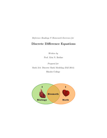
Reference Readings & Homework Exercises forDiscrete Difference EquationsWritten byProf. Erin N. BodinePrepared forMath 214: Discrete Math Modeling (Fall 2014)Rhodes College
Discrete Difference Equations11An Introduction to Discrete Mathematical ModelingThe field of mathematics provides many different means for modeling the world around us. Some mathematical toolsare more appropriate for modeling certain phenomenon and less appropriate for other phenomenon. In this course wefocus on how to use mathematics to simulate biological situations in which it is reasonable to assume the underlyingvariable of the model is discrete, that is, it can be written as a sequence of values. In contrast, the real number lineis continuous and for any two values a and b (no matter how close a and b are on the number line), we can alwaysfind another value that is between a and b. We may have to increase our precision to achieve this, but it can alwaysbe done. A sequence of discrete values is a set of points along the real number line. Thus, with a discrete model, weare assuming that we can ignore the space between the points.As one example, suppose we grow a cell culture in petri dish and measure the cell density (cells per unit area)every hour for 24 hours. This would create a sequence of 25 data points (if we include the initial cell density). Weknow that the cell culture is growing during the time between when we take our measurements, but measuring thepopulation each hour over the course of a day will give us a reasonable representation of how the culture grows overthe course of one day. Correspondingly, when we build a mathematical model to represent the growth of the cellculture, it is reasonable for the model to only predict how the culture grows from hour to hour. Thus, the underlyingvariable, time, is represented in the mathematical model as increasing in discrete, one hour increments.For another example, consider a population which breeds seasonally, that is, only once a year. If we wanted todetermine how the population size is changing over the course of many years, we could collect data to estimate thesize of the population at the same time each year (say shortly after the breeding season ends). We know that betweenthe times at which we estimate the population size some individuals will die and during the breeding season manynew individuals will be born, however, we ignore the changes in population size from day to day, or week to week, andlook only at how the population size changes from year to year. Thus, when we build a mathematical model of thispopulation, it is reasonable for the model to only predict the population size for each year shortly after the breedingseason. Here, the underlying variable, time, is represented in the mathematical model as increasing in discrete, oneyear increments.2A Motivating Example: Cell GrowthLet us consider an actual data set for the cell growth example described above. The data in Table 1 give the opticaldensity of an Escherichia coli (commonly referred to as E. coli ) cell culture measured every 30 minutes for 3 hours.The culture was grown in a nutrient solution at 37 C.Table 1: Optical Density of E. coli cell culture.Time (hours)0.00.51.01.52.02.53.0Cell Density (OD600 )0.0550.1200.2310.3600.5160.8211.300
Discrete Difference Equations2Escherichia coli : Abbreviated as E. coli, this bacteria lives in the lower intestines of endotherms (warm bloodedorganisms), including humans. There are variety of strains of E. coli many of which are part of the natural microbiomeof an endotherm’s intestinal tract. However, there are some strains of E. coli which can cause severe and adversereactions in their hosts including vomiting, fever, aches, and diarrhea (in humans).If we plot the data in Table 1 we obtain the graph in Figure 1. When we examine this data it would appear thatthe cell density is growing exponentially. How might weapproximate this sequence of cell densities using an algebraic expression, that is, a mathematical model?In general, when we want to describe a sequence mathematically, we want to express how the (n 1)th term inthe sequence, xn 1 is determined using previous n termsin the sequence, xn , xn 1 , xn 2 , . . . , x1 , x0 . Mathematically, we express the term xn 1 as a function of theprevious n terms, that isxn 1 f (xn , xn 1 , xn 2 , . . . , x1 , x0 ).(1)Equations which can be expressed in the form of Equa-Figure 1: Optical density of the E. coli cell culture measured every30 minutes over 3 hours.Table 2: Differences & ratios of consecutive terms of Sequence (2).tion (1) are known as discrete difference equations.nxn 1 xnxn 1 /xn00.0652.18For simplicity, let us assume that the next value in the10.1111.93cell density sequence can be determined using only the20.1291.56previous value in the sequence. Thus, xn 1 is a func-30.1561.43tion of xn , that is xn 1 f (xn ), which is called a first40.3051.59order difference equation. Often we can determine50.4791.58the relationship between two consecutive terms in a sequence, xn and xn 1 , by examining either the difference or ratio between those two terms, that is xn 1 xn orxn 1 /xn , respectively. For the data presented in Table 1, let xn represent the cell density of the nth data point,where n 0 denotes the data point at 0 hours, n 1 denotes the data point at 30 minutes, etc. Thus,x0 0.055, x1 0.120, x2 0.231, x3 0.360, x4 0.561, x5 0.821, x6 1.300,(2)where the underlying variable, time, is represented as increasing in discrete 30 minute increments. Table 2 showsboth the difference and ratio of consecutive terms in the sequence representing the cell density data from Table 1.The difference between consecutive terms in the sequence are increasing as n increases. However, with the exceptionof the first two ratios, the ratios of consecutive terms appears to remain relatively constant as n increases. Supposethe ratios of consecutive terms were constant with a value c as n increased, thenxn 1 c xn 1 cxn ,xn
Discrete Difference Equations3and thus we have written xn 1 as a function of xn (where f (xn ) cxn ). Given that the ratios of consecutive termsshow little fluctuation, we might assume that the fluctuations we see are due to measurement error (either by thespectrophotometer used to measure the optical density or by the human taking the measurements). If we assumethat the ratios of consecutive terms would be constant if not for measurement error, then what would be the valueof c? We could use the average (mean value) of all of the ratios: 1.7. We could also use the average of the last fourratios: 1.5. Thus, we have two options for our model:xn 1 1.7xn (model 1), and xn 1 1.5xn (model 2).How do we decide which model is “better”? First, whatdoes it mean for one model to be better than anothermodel? In this case, we are interested in seeing whichmodel is better able to accurately reproduce the data.When we use model 1 with x0 0.055, we generate thesequencex0 0.055, x1 0.094, x2 0.159, x3 0.270,x4 0.459, x5 0.781, x6 1.328.(3)When we use model 2 with x0 0.055, we generate thesequenceFigure 2: Optical density of the E. coli cell culture measured every30 minutes over 3 hours (dotted grey), and estimated optical densityusing model 1 (solid blue) and model 2 (dashed red).x0 0.055, x1 0.083, x2 0.124, x3 0.186,x4 0.278, x5 0.418, x6 0.626.(4)Figure 2 show a plot of the sequence of the original data (gray) against the sequences generated by model 1 (blue)and model 2 (red). Which model appears to approximate the data better? It would appear that model 1, thoughnot perfect, does a better job approximating the data.Optical Density: How does one “count” the number of cells in a cell culture? The number of cells in a culture couldbe quite large (on the order of millions or billions). It would indeed be a tedious task to sit down and count the totalnumber of cells in such a culture. In fact, if the culture is growing (the number of cells are increasing), by the timeyou counted the first 200 cells, the size of culture would likely have changed. Instead of counting the number of cellsin a culture of volume V , we sample the culture, that is, we take a representative portion of the culture and countthe number of cells in the sample. Suppose the sample has Ns cells, and a volume of Vs . If we assume that the celldensity (cells per unit volume) are the same in the whole culture as in the sample, then N/V Ns /Vs , where N is thetotal number of cells in the sample. Thus, N V (Ns /Vs ). The ratio Ns /Vs is proportional to the optical density (i.e.Ns /Vs a · OD where a is a constant and OD is the optical density) and is measured using a spectrophotometer. Thesample is placed in a cuvette (essentially a rectangular test tube) and the spectrophotometer shines a beam of light (ofa specified wavelength) through the cuvette. The denser the cell culture, the less light will shine through the cuvette.By measuring the amount of light that does not make it through the cuvette (light that scatters due to the cells inthe cuvette), the spectrophotometer measures the optical density of the cell culture sample. The intensity of the lightscattering, and thus the measure of optical density, depends on the wavelength of light being used. The wavelengthof light used, measured in nanometers (nm), is denoted by a subscript of OD. Thus, an optical density measure takenusing a light with wavelength 600 nm is indicated by OD600 .
Discrete Difference Equations34Discrete Exponential Growth ModelThe equation xn 1 axn is known as the discrete exponential growth model , and sequences generated byfunctions of the form xn 1 axn are known as geometric sequences. Given a value of x0 , thenx1 ax0x2 ax1 a(ax0 ) a2 x0x3 ax2 a(a2 x0 ) a3 x0.xn axn 1 an x0 .The equationxn an x0(5)is known as the general solution or closed form solution of the equation xn 1 axn . Note, for Equation 5, ifyou know the initial value of the sequence, x0 , you are able to determine the value of the nth term of the sequencewithout iterating through all n terms (which could be tedious for large n).Suppose a 1, then xn 1 axn xn . This means that when a 1 the (n 1)th term in the sequence is alwayslarger than the term that came before it, the nth term. We describe such a sequence as an increasing sequence.In the example where xn represents the cell density of the E. coli population at time step n, a 1 implies that thecell culture is growing; specifically, it is becoming more dense. By examining the closed form solution xn 1 an x0 ,we can see that as n becomes increasingly large (denoted by n ), the value of an if a 1. Thus, as weallow n to increase towards infinity, the values of the sequence always increase towards infinity. This makes intuitivesense since this discrete difference equation models exponential growth.If a 1, then xn 1 axn xn which means the (n 1)th term in the sequence is always smaller than the termthat came before it, the nth term, and thus we have a decreasing sequence. By examining the close form solutionxn 1 an x0 , we can see that as n , an 0 when a 1. This also makes intuitive sense since the amount of xis being reduced by some proportion with each increment of n. Note, in the special case when a 1, xn 1 xn forall n, and thus every value in the sequence is the same.Let a 1 r, then the discrete exponential growth model becomesxn 1 (1 r)xn xn rxn .(6)The red term, xn , represents the amount of x at time step n, and the blue term, rxn , represents a proportion of xat time step n. Thus, the amount of x at time step n 1 is the amount of x at time step n plus a proportion of xat time step n. Notice if r 0 (which corresponds to a 1), then we will be subtracting a proportion of x at timestep n.If, for example, we knew a population was increasing 3% each year, we could represent the population size asxn 1 xn 0.03xn 1.03xn ,where xn represents the population size at year n. Note that this difference equation produces an increasing sequence
Discrete Difference Equations5and thus, xn as n . If, on the other hand, the population was decreasing by 3% each year, then we wouldrepresent the population size asxn 1 xn 0.03xn 0.97xn ,where xn represents the population size at year n. This difference equation produces a decreasing sequence and thus,xn 0 as n .Table 3: Difference quotients of consecutive terms of Sequence (2).Note that Equation (6) can be rewritten asxn 1 xn rxn ,(7)n(xn 1 xn ) /xn01.18210.925which denotes the difference in the amount of x from time n to time n 1.The equation in this form reveals why we refer to these types of equations as20.558difference equations. Note, the change in x over one time step is a proportion30.433(r) of the amount at the previous time step (xn ). Thus, we say “the change is40.591x is proportional to the amount of x.” Furthermore, if we rewrite Equation (7)50.583asxn 1 xn r,xn(8)then we have a direct way to estimate the value of r for a model. Table 3 shows the values of the difference quotientsin Equation (8) for n 0, 1, . . . , 5. If we average the values in the second column of Table 3, we obtain 0.619 0.7as an estimate of r. Note, this concurs with the value of a 1.7 since a 1 r.Example 1.We determined that a reasonable model for the density of E. coli cells given the data presented in Table 1 isxn 1 1.7xn .(a) Find the general solution to this difference equation.(b) Does this difference equation model produce an increasing or decreasing sequence?(c) Given this model, what cell density would we predict at 6 hours? at 10 hours? at 24 hours? Do these values make biological sense?(d) What happens to the population of E. coli cells as n ? Is this biologically reasonable?The solutions to this example will be worked in class.Example 2.The Forest and Wildlife Research Center at Mississippi State University measured the survival and mortality rates of bobcats (Lynxrufus) in and near the Tallahala Wildlife Management Area through their Carnivore Ecology Research Project [8]. They studied 68bobcats (28 males and 40 females) and found that the mean annual survival was 75% for males and 84% for females.(a) Use a discrete difference equation model to express how many male bobcats (of the original 28) are still alive at year n. Assume thatthere are 28 male bobcats at year n 0. Express the model in closed form solution.(b) Use a discrete difference equation model to express how many female bobcats (of the original 40) are still alive at year n. Assumethat there are 40 female bobcats are year n 0. Express the model in closed form solution.(c) Both models generate decreasing sequences. Which is decreasing more quickly?(d) What is the first year in which there will be no male bobcats left (i.e. less than 1 male bobcat) of the original 28? What is the firstyear in which there will be no female bobcats left of the original 40?The solutions to this example will be worked in class.
Discrete Difference Equations6Exercise 1 – Wild HaresSuppose a population of wild hares increases by 12% each year, and there are currently 200 hares. Let xn be the number of hares in thepopulation at year n.(a) Find the difference equation representing xn 1 as a function of xn .(b) Find the general solution to the difference equation found in (a).(c) Find the number of hares in the population 6 years from now.(d) What happens to the population of hares as n ? Is this biologically reasonable?Exercise 2 – Elk HerdLet xn be the number of adult elk in a newly introduced elk herd in a wildlife management area in the Cumberland Mountains inTennesseee. There are currently 50 adult elk in the population.(a) Suppose the number of adults in the population increases by 10% each year. Use a discrete difference equation model to express howthe number of adult elk in the population at year n (express your model in the closed form solution). Does your model generate anincreasing or decreasing sequence? Determine how many adult elk are in the population after 20 years.(b) Suppose that the probability that an adult elk survives in a given year is 90%. Use a discrete difference equation model to expresshow many of the originally introduced adult still alive at year n (express your model in the close form solution). Does your modelgenerate an increasing or decreasing sequence? Determine how many of the originally introduced elk are still alive after 20 years.Elk live, on average, 15 years in the wild. Does your answer make biological sense?Exercise 3 – Treating Heart DiseaseDigoxin is used in the treatment of heart disease. Doctors must prescribe an amount of medicine that keeps the concentration of digoxin inthe bloodstream above a minimum level of effectiveness without exceeding the maximum level for safety (these levels vary among patients).For an initial dosage of 0.5 mg in the bloodstream, the table below shows the amount of digoxin (x) remaining in the bloodstream of aparticular patient after n days.Time (days)012345678Digoxin a) Suppose the amount of digoxin in the bloodstream of the patient can be modeled using xn 1 axn , where xn is the amount ofdigoxin (in mg) in the bloodstream on day n. Use the ratio of consecutive terms in the sequence to determine the value of a.(b) Express your model in its closed form solution.(c) In this patient the digoxin is effective if it remains above 0.01 mg, however digoxin toxicity occurs when the amount of digoxin inthe bloodstream exceeds 0.6 mg. When would you recommend this patient take his or her next dose of digoxin.Note, we will revisit this example and the idea of timing between doses once we have explored some more sophisticated differenceequation models.
Discrete Difference Equations47Discrete Model with Exponential & Constant GrowthIn the discrete exponential growth model, the change in x (represented as xn 1 xn ) was proportional to x (that isxn ), thus we had the equationxn 1 xn rxn ,where r is the proportionality constant which represents the rate of change. However, what if the change is notproportional, but constant, that is what ifxn 1 xn b,(9)where b is a constant. Equation (9) can be rewritten asxn 1 xn b,(10)and we will refer to this model as the constant growth model . The sequence generated by Equation (10) is knownas an arithmetic sequence. As with the discrete exponential growth model, we can find a closed form solution ofthe constant growth model. Given a value for x0 , thenx1 x0 bx2 x1 b (x0 b) b x0 2bx3 x2 b (x0 2b) b x0 3b.xn x0 nb.Note, if b 0 then the values of xn increase as n , but if b 0 then the value of xn decrease as n . Inparticular, the values of xn can become negative if b 0 and n is large enough, even if x0 0. This may or may notbe biologically reasonable depending on what is being modeled.In general, we will not use the constant growth model on its own, but in combination with the exponential growthmodel. In this section we will examine a variety of models (known as first order linear difference equations) ofthe formxn 1 axn {z}exponentialgrowth b . {z}(11)constantgrowthBefore we look at specific biological phenomenon which can be modeled using Equation (11), we shall derive theclosed form solution (see below) and discuss the notion of the model begin at equilibrium and how to determine thelong term behavior of a model (see the next section). Given x0 , then the closed form solution is derived asx1 ax0 bx2 ax1 b a [ax0 b] b a2 x0 (a 1)b ax2 b a a2 x0 (a 1)b a3 x0 a2 a 1 b. an x0 an 1 · · · a2 a 1 b.x3xn
Discrete Difference Equations8This is a way to express the closed form solution, but it seems rather unwieldy. It would be nice if that (n 1)thorder polynomial in terms of a weren’t mucking up the equation. With some good old fashioned polynomial longdivision (think back to your fondest memories of Algebra II), it can be shown that1 an (1 a) 1 a a2 · · · an 1 1 an 1 a a2 · · · an 1 ,1 aprovided a 6 1. Thus, we can rewrite the closed form solution asxn an x0 1 anb,1 awhich feels much more manageable as an equation, and will be easier to work with as we progress forward. Noticeif a 1, then Equation (11) reduces to the constant growth model represented by Equation (10).5Equilibria & Long-Term BehaviorEquilibriaThe term equilibrium refers to being in a state of balance and remaining as you are. In the case of discrete differenceequation models, a number x is called an equilbrium point or fixed point of the difference equation xn 1 f (xn )if x f (x ). Let us examine this concept for the few discrete difference equation models we have encountered sofar.Exponential Growth Model · Recall the exponential growth model has the form xn 1 axn , where a is aconstant. The model will be in equilibrium when x ax which can only occur if a 1. Thus, when a 6 1, thereis no fixed point for the model which makes sense because the values of xn are either always increasing (a 1) oralways decreasing (a 1). When a 1, xn x0 for all n.Constant Growth Model · Recall the constant growth model has the form xn 1 xn b, where b is a constant.The model will be in equilibrium when x x b which can only occur if b 0. Thus, when b 6 0, there is nofixed point for the model which make sense because the values of xn are either always increasing (b 0) or alwaysdecreasing (b 0). When b 0, xn x0 for all n.Exponential & Constant Growth Model· Recall the difference equation model with exponential andconstant growth has the form xn 1 axn b, where a and b are constants. The model will be in equilibriumwhenx ax b (1 a)x b x b.1 aThis is different from the previous two examples because this does not require that a and b take on certain valuesfor the model to have a fixed point, and the fixed point is not necessarily the initial condition x0 . When we examinethis model as it pertains to different biological phenomenon, we will see the different ways in which we can interpretthe meaning of the equilibrium value x .
Discrete Difference Equations9Long-Term BehaviorWhen you are examining the features of a model xn 1 f (xn ), it if often useful to know what happens to the modelas n . This is known as the long-term behavior of the model. We already examined the long term behaviorof the exponential growth model and constant growth model under various parameter scenarios (a 1, a 1, a 1for the exponential growth model, and b 0, b 0, b 0 for the constant growth model).It turns out there is another, more visual way to examine the long-term behavior of these models called cobwebdiagram analysis. On the xn , xn 1 plane (where xn is the horizontal axis and xn 1 is the vertical axis), we plotxn 1 f (xn ) and xn 1 xn . On the xn (horizontal) axis, locate x0 . Draw a vertical line from x0 on the horizontalaxis to the xn 1 f (xn ) curve. Your height on the vertical axis now represents x1 . To locate x1 on the horizontalaxis, draw a horizontal line from (x0 , x1 ) to the xn 1 xn line; you are now at (x1 , x1 ). Then, (starting withn 1)1. Draw a vertical line from (xn , xn ) to the curve xn 1 f (xn ); you are now at (xn , xn 1 ).2. Draw a horizontal line from (xn , xn 1 ) to the line xn 1 xn ; you are now at (xn 1 , xn 1 ).3. Repeat steps 1 & 2 with increasing values of n as many times as needed to see a pattern.Figure 3 shows what this looks like for the discrete exponential growth model when (a) a 1 and (b) a 1. Ineach graph the blue curve represents xn 1 axn and the black line represents xn 1 xn . The dotted red line showthe “cobwebbing”. In Figure 3a (where a 1) we can see that the cobwebbing (dotted red line) steps up and awayfrom x0 as n increases. This is because the values of xn (and thus xn 1 ) are increasing as n increases. In Figure 3b(where 0 a 1) we can see that the cobwebbing (dotted red line) steps down towards (0, 0) as n increases.This method may seem like overkill for these simple difference equations but it will be very handy for analyzing thelong-term behavior of xn 1 axn b.(a) a 1(b) a 1Figure 3: Cobweb diagrams for the discrete exponential growth model for (a) a 1 and (b) a 1.Note that for the difference equation model with exponential and constant growth, xn 1 axn b, it is a littleharder to determine the long term behavior because their are two parameters, a and b, and the relative size and signof each parameter will have a bearing on what happens to the values of xn as n . Suppose x0 0. If a 1 andb 0 we would expect the population to grow, and if a 1 and b 0 we would expect the population to decline.
Discrete Difference Equations10And indeed, in both cases we are correct as shown in the cobweb diagrams depicted in Figures 4a and 4b. Noticethat in the case where a 1 and b 0, the values of xn quickly become negative despite the fact that x0 0.(a) a 1, b 0(b) a 1, b 0(c) a 1, b 0(d) a 1, b 0Figure 4: Cobweb diagrams for xn 1 axn b.Now, suppose a 1 and b 0. What do we expect to happen in this case. The value of a will cause a decreasewhile the value of b will cause an increase. If we examine the cobweb diagram in Figure 4c we see that the linesbbb, 1 a,xn 1 xn and xn 1 axn b cross in the first quadrant at the point 1 a. Notice if we choose x0 1 athen xn for all n, and thus x b1 athe values of xn increase towardsb1 a .b1 ais an equilibrium point. If we choose x0 such that 0 x0 If we choose x0 b1 a ,then the values of xn decrease towardsmatter what value of x0 we choose, as n the values of xn approachb1 a .b1 a .b1 a ,thenThus, noSince the sequence of values approachthe equilibrium point, we classify the fixed point as a stable equilibrium.Lastly, suppose a 1 and b 0. If we examine the cobweb diagram in Figure 4d we see again that the linesbbbxn 1 xn and xn 1 axn b cross in the first quadrant at the point 1 a , 1 a , and that if we choose x0 1 a,then xn b1 afor all n, and thus x b1 ais an equilibrium point. However, if we choose x0 such that 0 x0 then the values of xn decrease towards . If we choose x0 b1 a ,then the values of xn increase towards . Inthis case, not matter what value of x0 we choose, with the exception of x0 away fromb1 a ,b1 a ,b1 a ,as n the values of xn moveand we classify this type of fix point as an unstable equilibrium.
Discrete Difference Equations11Example 3.Consider a lake fish population which increases on average by 20% annually. Each year, fishing on the lake is allowed until 1200 fish arecaught. Thereafter, fishing is banned. Currently, there are 12,230 fish in the lake.(a) Write a difference equation for the lake fish population and find the general solution.(b) How many fish are in the lake after 5 years?(c) If the resource managers of the lake wanted the population to remain constant each year, what level of harvesting should they allow?Note, this value is referred to as the maximum sustainable yield (MYS) .(d) How is the maximum sustainable yield related to the equilibrium value of this system?The solutions to this example will be worked in class.Example 4.Consider a lake fish population whose yearly birth rate is 1.5 and whose yearly death rate is 0.7. Each year, fishing on the lake is alloweduntil 1200 fish are caught, thereafter, fishing is banned. Currently, there are 12,230 fish in the lake. If the resource managers of the lakewish to keep the fish population constant from year to year, how many fish are needed to stock the lake each year?The solutions to this example will be worked in class.Exercise 4 – BuffaloA population of buffalo increases in size by about 10% each year. Let xn be the population count after n years. Suppose that huntingallows h buffalo to be removed from the herd each year.(a) Find an expression for xn in terms of n if x0 1000 and h 20.(b) Will terms in the sequence generated by the expression you found in (a) ever be negative?(c) Determine a value for h such that the population with x0 1000 remains at equilibrium.Exercise 5 – TroutSuppose that in a trout population increases its own numbers by 10% each year. After the births occur each year, 100 young trout areadded to the population in an effort to build up the population. Let xn denote the size of the population after n years, and assumex0 1000.(a) For what n does xn 2000 first occur?(b) Suppose that after the time found in part (a) the lake is not longer stocked. How many trout should the lake managers allow to becaught each year if they want the trout population to remain stable (i.e., at equilibrium). Hint: Let create a new first order lineardifference equation where x0 is the size of the population at the value of n found in part (a) rounded to the nearest whole fish.6Drug Dosing & PharmacokineticsPharmacokinetics is a branch of pharmacology which quantifies how the concentration of a substance administeredto a living organism declines over time (from the moment it is introduced to the body/organism to the point at whichit is entirely eliminated from the body). You have already seen one example of pharmacokinetics in Exercise 3 whereyou expressed the decay of digoxin (a drug used in treated heart disease) as a discrete exponential decay model. Inthat example, only once dose was given. In this section we examine what occurs to the concentration of a drug inthe body when we give successive doses of the same drug over some period of time.
Discrete Difference Equations12For many drugs administered intravenously, the amount of drugin the body after a dose of size b administered at time t 0isx(t) be
Discrete Di erence Equations 1 1An Introduction to Discrete Mathematical Modeling The eld of mathematics provides many di erent means for modeling the world around us. Some mathematical tools are more appropriate for modeling certain phenomenon and less appropriate