Transcription
1STA1510 (BASIC STATISTICS) AND STA1610 (INTRODUCTION TO STATISTICS)NOTES PART 1Dear student,I pray that this information finds you in good health. These notes are written an integral partof Unisa’s student support programme – a programme that seeks to bridge the distancebetween the student, the study material and the lecturers. In this work we discuss chapter 1to chapter 7 of the prescribed text book. Understanding this work will help you cover all thecontent assessed in assignment 1.Please note that parts of these notes are extracts from the prescribed text book, the studyguide, other statistics sources and large proportion is based from the lecturer’s synthesis.This means that many real life examples used are based on the lecturer’s understanding andsubject to change. In a situation where you do not understand or you disagree with theauthor please share your view with us. I trust that this information will be helpful andrewarding.Rajab SsekumaLecturerDepartment of StatisticsTel: 27 12 429 6634email: ssekur@unisa.ac.za
2STUDY UNIT 1Key questions for this unitWhat is Statistics?What is the difference between Population and a Sample?What is the difference between a parameter and a Statistic?Distinguish between Qualitative and Quantitative variables.Distinguish between Nominal and Ordinal variables.Distinguish between Discrete and Continuous variables.Distinguish between Scale and Ratio variables.DEFINITIONSStatistics is a way to get information from data. In other words, statistics is a tool ‘’like atoolbox’’ used to extract information form collected data. Statistics has two main branches;Descriptive and Inferential statistics.Descriptive statistics: This deals with methods of organising, summarizing and presentingdata in a convenient and informative way. In descriptive statistics, we use graphs, tables,numerical measures like mean, range, median mode etc to summarise data.Inferential statistics: This is a body of methods used to draw conclusions or inferences aboutcharacteristics of population based on sample data.A population: This is the group of all items of interest to a statistics practitioner. It could bepeople, cars, house etc. It is frequently very large and may, in fact, be infinitely large.A sample: This is a set of data drawn from the studied population. In other words, a sampleis part of a population.A parameter: Any descriptive measure of a population is a parameter. Examples ofparameters include; population size (N ) , population variance ( sigma-squared σ 2 ),population standard deviation (sigma σ ). In other words, any numerical summary from apopulation is a parameter.A statistic: Any descriptive measure of a sample is a statistic. Examples include; sample size(n) , sample variance ( s 2 ), sample standard deviation ( s ). In other words, any numericalsummary from a sample is a statistic.
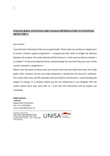
3TYPES OF VARIABLES1.1Introduction to this study unitThis unit introduces the concepts of types of variables. There arebasically two types of variables in statistics; Qualitative (think in termsof quality of life) and Quantitative (if you quantify something you couldcount it).Qualitative variables are then classified into nominal andordinal variables. Quantitative variable can be classified into discreteand continuous variables. Once you know your variable is quantitative,it helps to ask yourself if you have actually counted (then discrete) ormeasured (then continuous), when you gather the values.The diagram below is a mind map of what we shall focus on in thissection. Please note that though we have to know how to differentiatebetween variables, questions in this section are set in application formas we shall see when we get to examples and exercises.1.2Qualitative Vs Quantitative variables1.2.1 Qualitative Variables (Categorical Variable)Also known as categorical variables, qualitative variables are variables with no natural senseof ordering. They are therefore measured on a nominal scale. For instance, hair colour(Black, Brown, Gray, Red, Yellow) is a qualitative variable, as is name (Adam, Becky,
4Christina, Dave . . .). Qualitative variables can be coded to appear numeric but theirnumbers are meaningless, as in male 1, female 2. Variables that are not qualitative areknown as quantitative variables.1.2.2 Quantitative VariablesQuantitative variables are variables measured on a numeric scale. Height, weight, responsetime, subjective rating of pain, temperature, and score on an exam are all examples ofquantitative variables. Quantitative variables are distinguished from categorical (sometimescalled qualitative) variables such as colour, religion, city of birth, sport in which there is noordering or measuring involved.1.3 Nominal Vs Ordinal variables1.3.1 Nominal VariablesA nominal variable has values which have no numerical value. As a result the order orsequence of nominal variables is not prescribed. Examples of nominal variables are gender,occupation.1.3.2 Ordinal variablesAn ordinal variable is similar to a categorical variable. The difference between the two isthat there is a clear ordering of the variables. For example, suppose you have a variable,economic status, with three categories (low, medium and high). In addition to being able toclassify people into these three categories, you can order the categories as low, mediumand high.Please note that the major difference between ordinal and nominal is that order isconsidered to be important in ordinal variables than in nominal variables.1.4 Discrete Vs Continuous variables1.4.1 Discrete variablesVariables that can only take on a finite number of values are called "discrete variables." Or Avariable that takes values from a finite or countable set, such as the number of legs of ananimal. All qualitative variables are discrete. Some quantitative variables are discrete, suchas performance rated as 1,2,3,4, or 5, or temperature rounded to the nearest degree.1.4.2 Continuous variablesA continuous variable is one for which, within the limits the variable ranges, any value ispossible. For example, the variable "Time to solve a mathematical problem" is continuoussince it could take 2 minutes, 2.13 minutes etc. to finish a problem.I like telling my students to look at discrete variables as countable variables with gaps inbetween say the number of students in a discussion class, and to look at continuous
5variables as countable with decimal point like money R5.13, time, height e.t.c. Please notethat this is not a standard difference between the two but a personal option.1.5 Interval Vs Ratio variables1.5.1 Interval variablesAn interval variable is similar to an ordinal variable, except that the intervals between thevalues of the interval variable are equally spaced. For example, suppose you have a variablesuch as annual income that is measured in Rand, and we have three people who makeR10,000, R15,000 and R20,000. The second person makes R5,000 more than the first personand R5,000 less than the third person, and the size of these intervals is the same. If therewere two other people who make R90,000 and R95,000, the size of that interval betweenthese two people is also the same (R5,000).1.5.2 Ratio variablesA variable with the features of interval variable and, additionally, whose any two valueshave meaningful ratio, making the operations of multiplication and division meaningful.Now that we are familiar with the definitions, we can take example on how this unit isexamined. Please remember that we examine their applications to real life situations in mostcases.Example 1Which one of the following statements is incorrect?(1) The number of students who attended both discussion classes in 2010 is adiscrete variable.(2) Your marital status is a discrete variable.(3) Whether one does poor, fair or good in an assignment is an ordinal variable.(4) The amount of your student loan is a continuous variable.(5) Your status as a full-time student is a nominal variable.
6SolutionThe number of students who attended both discussion classes in 2010 a discretevariable (correct).1.Maritial status (married, not married, single or divorce) is a nominal .Example 2The owner of fancy foods chooses a random sample of six people who are at his shop. Heasks them a few questions that are summarised as follows:SexAgeMethod of payment Satisfaction of service1 Male1 under 201 cashrating2 credit card1 bad2 Female2 20 to 403 private account2 average3 41 to 603 good4 over 604 very good221312141121243313321323Consider the following statements:A: Method of payment is a quantitative variable.B: The youngest person is male, paid with a credit card and found the service bad.C: 50% of the people said the service was good.D: 50% of the males were under 20.E: The oldest person interviewed said the service was very good.The correct statements(s) is/are(1) Only B(2) C and D(3) B and C(4) C,D and E(5) A and C
7Option (1). The youngest person is male, paid with a credit card and found the service bad.Sex1 MaleAge1 under 20Method of payment2 credit cardSatisfaction of service rating1 badSELF ASSESSMENT EXERCISE – TEST YOUR KNOWLEDGEQuestion 1Which one of the following statements is incorrect?(1) Measures for a sample are called statistics while measures for a population arecalled parameters.(2) Your marital status is an ordinal variable.(3) Whether one does poor, fair or good in an assignment is an ordinal variable.(4) The amount of your student loan is a continuous variable.(5) The starting salary of MBA graduates is a quantitative variable.Question 2Which of the following variables is a qualitative variable?(1) The most frequent use of your microwave oven (reheating, defrosting, warming,others).(2) The number of consumers who refuse to answer a telephone survey.(3) The number of mice used in a maize experiment.(4) The winning time for a horse running in a Derby.(5) Weight of a new-born baby.Question 3Which one of the following is a discrete variable?(1) Writing skills of new employees, classified as bad, fair, good and excellent.(2) A student’s yes/no response to a question in a campus newspaper.(3) The combined weight of parcels sent from a certain post office during a week.(4) The starting salary of a medical doctor.(5) The number of students who attended a discussion class.
8Question 4Which of the following statements is incorrect?(1) The number of registered arms dealers in a certain province is a discrete variable.(2) Your choice of car brand is a nominal variable.(3) The average mark of statistics students in the exam is a qualitative variable.(4) The number of building permits for new single-family housing units is a discrete variable.(5) The opinion of TV viewers on a new program (bad, indifferent, good) is an ordinalvariable.SOLUTIONS TO SELF ASSESSMENT EXERCISESQuestion 1Alternative 2. Your marital status is a nominal variable.Question 2Alternative 1. The most frequent use of your microwave oven (reheating, defrosting,warming, others) is a qualitative variable.Question 3Alternative 5. The number of students who attended a discussion class is a discrete randomvariable.Question 4Alternative 3. The average mark of statistics students in the exam is a quantitative variable.
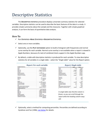
9STUDY UNIT 22 DESCRIPTION OF DATAKey questions for this unitDistinguish between Qualitative and Quantitative data.How would you represent qualitative data both numericallyand visually?How would you represent qualitative data both numericallyand visually?Interpretation of a frequency distribution and the stem-andleaf diagram2.1Introduction to this study unitNow that we know that in data can be classified in two ways, that is,qualitative and quantitative. We pose a question, how would wedescribe data? Description of data can be done in two ways: numericallyand visually as shown in the following flow diagramThe diagram below is a mind map of what we shall focus on in thissection. Please note that questions in this section are most theoretical.In the past mostly examiners have focused on the stem-and –leafdiagram.
102.1 Qualitative Data:Remember in study unit 1 we classified qualitative as categorical data. Think in terms ofgender, say, you have a class of female and male students.2.1.1 Numerical SummaryTo summarise this data numerically, you would perhaps first think of how many are femaleor male (frequency), what percentage are male or female, what is the fraction (Ratio) ofmale to female which is the relative frequency. There is not too much we can do in terms ofsummarising qualitative data numerically.2.1.2 Visual SummaryVisually if data is qualitative, in most cases we use the bar chart or the pie chart to representit. The figures below are examples of Bar chart and Pie charts respectively.2.2 Quantitative dataFrom study unit 1, we classified quantitative data as countable or measurable on a numericscale. In this case think in terms of salaries.2.2.1 Numerical SummaryIf you are to access employees salaries, you would first look at the average (mean) salary,the middle(median) salary, the most occurring (mode) salary, the variance (see study unit 3),the standard deviation (see study unit 3), the range , kurtosis, correlation, skewness. In briefmost of the statistical analysis is done on quantitative data.
112.2.2 Visual SummaryVisually if data is quantitative, we use the histogram, the frequency polygon, the stem-andleaf diagram, scatter plot, line graph and the box-and-whisker plot to represent it. With theexception of the stem-and-leaf diagram, the reset are examinable theoretically. If theexaminer wants to examine the features of any diagram, it will be drawn for you.Example 3Which one of the following statements is incorrect?(1) A bar graph cannot be used for two categorical variables.(2) Adjacent rectangles in a histogram share a common side.(3) A stem-and –leaf plot provides sufficient information to determine whether adataset contains an outlier.(4) Box plots display the centre, spread and outliers of a distribution.(5) A histogram is better than a box plot for evaluating the shape of a dataset.SolutionOption 1:A bar graph can be used for two categorical variablesExample 4The following table gives the cumulative relative frequency of the mass of 100 youngsters:Class intervalCumulative relativefrequency19.5 29.50.0429.5 39.50.1839.5 49.50.3549.5 59.50.6059.5 69.50.800.9469.5 79.579.5 89.51.00Which of the following statements is incorrect?(1) The interval 49.5-59.5 has the largest number of observations.(2) There are 35 youngsters having a mass of more than 49.5 kg.(3) The interval 39.5-59.5 has 42 observations.(4) 94% of the youngsters have a mass of less than 79.5 kg.(5) The interval 19.5-29.5 has 4 observations.
12SolutionClass interval19.5 29.529.5 39.539.5 49.549.5 59.559.5 69.569.5 79.579.5 89.5Cumulative 14172520146Option (1) CorrectThere are 25 youngsters in the interval 49.5 59.5Option (2) IncorrectThere are (25 20 14 6) 65 youngsters having a mass of more than 49.5 kgOption (3) CorrectThe interval 39.5 59.5 39 has (17 25) 42 observations.Option (4) CorrectThe number of youngsters with less than 79.5 kg is (4 14 17 25 20 14) 94.94The percentage is therefore 100 94%100Option (5) CorrectThe interval 19.5 29.5 has 4 observations
13STUDY UNIT 3In this study unit we discuss the following1. Measures of location / measures of central tendency.2. Measures of spread / measures of dispersion3. Quartiles, Box plots and Percentiles4. Measures of linear relationships3.1 Measures of central tendency / Measures of locationThese include the mean, the median and the mode.3.1.1 The mean / AverageThe mean (averages) is calculated by summing all the observations and dividing by theirnumber. Calculation of the mean depends on the source of the data. This can either be thepopulation or the sampleExample:Calculate the mean following sample data: 29, 39, 43, 52, 39The sample meannx xi 1in29 39 43 52 39 5202 5 40.4
143.1.2 The medianThe median of the data set is the middle value of an ordered data set. Before calculating themedian, the data set has to be arranged in order (either ascending or descending).Please note that:(i) If the data set is odd in number, its quite easy to identify the middle value which, isthe median.For example: consider the following data set: 29, 39, 52, 43, 39(ii) If the data set is even in number, the median is the average of the two middle value.For example: Consider the following data set; 29, 43, 39, 39, 56, 523.1.3 The modeThe mode is the most occurring observation in a data set. Or we can say the observationwith the highest frequency. For example in the following data set: 29, 39, 39, 43, 52, 56,the mode is 39.Please note that:(i) It’s possible for a data set not to have a mode. E.g: there is no model in the followingdata set 29, 39, 43. However, this does not mean that the mode is zero. If you saythat mode is zero, it implies that the value (0) occurs most, which is not true inthis case.(ii) It’s also possible for the data set to have two modes. Such a data set is called abimodal data set. Plotting such a data set will lead to two peaks as shown belowExample 5The following stem-and-leaf display is for a set of values where the stem is formed by theunits and the leaf represents the decimal digits:
15Which of the following statements is incorrect?(1) The number of values larger than 4.0 is 12(2) The median of this data set is 3.7(3) 20% of the values lie between the values 2 and 3(4) The mode of the data set is 3.6(5) The sixth smallest value in the data set is 2.8SolutionOption (2)3.7 3.8Median 3.7523.2 Measures of Dispersion / Measures of Spread3.2.1 RangeThis is perhaps the most easiest to calculate. The range is the difference between the largestand the smallest observation of a data set.3.2.2 VarianceCalculation of the variance depends on the source of the data, which is either from apopulation of the sample.3.2.3 Standard deviationThe standard deviation is the positive square root of the variance.Calculation of the standard deviation also depends on the source of the data, which is eitherfrom a population of the sample.
16Please note that the mean, the standard deviation and the variance can also be excuteddirectly from any scientific calculator. If you are using the SHARP EL531WH advanced D.A.Llike mine, you follow the following steps.1. Set you calculator in Stat 0 mode as follows; Press mode, press 1, press 0. You willhaveon your screen2. Enter the data set as follows. E.g. Consider the data set as follows: 42, 45, 48, 79The m button next to the STO button stores the observations in the memory of yourcalculator. Your will haveThis means that you have 4 observations stored in the memory.3. To get the mean, press RCL and 4. On the top of number 4, there is a small x , whichstandard for the mean. It’s green in colour and to use green keys we either use RCL(recall) or use ALPHA. You will haveThis is equivalent to calculating the mean manually as;nx xi 1in42 45 48 79 4214 4 53.54. To get the standard deviation, we press RCL(recall) , then press number 5. Thestandard deviation is the small green s x on the top of number 5. You will haveThis will have saved you time spent in using the following formula.
17ns (xi 1 x)2in 12(x) 1 2 x n n 1 (214)2 1 12334 4 4 1 1[12334 11449]3 (885)3 295 17.17556404Please remember that x2 42 2 45 2 48 2 79 2 12334 . We clearly see that working itout manually takes a lot of time and we are likely to make mistakes.5. To get the variance using our calculator, we just need to square the answer of thestandard deviation. After pressing RCL number 5, press x 2 , then press equal sign.You will haveOtherwise we have to square (17.17556404) 295 . Please remember that sinceThen3.2.4 Coefficient of variationThis measures the scatter in the data relative to the mean. In many Statistics book, itsexpressed as a a percentage. The coefficient of variation also depends on the source of thedata.
183.3 Quartiles Box plot and Percentiles3.3.1 The first (lower), the second (median) and the upper (third) quartilesFor purposes of this module, we shall only discuss the quartiles. The word quartile perhaps 1 comes from quarter . This means that quartiles divide a data set into four equal parts as 4 follows:The calculation of the quartiles requires to first arrange the data set in order, preferably inascending order. Once the data is arranged in order, we then obtain the position of aparticular quartile as follows: n 1 (i) The location/position of first (lower) quartile is given by where n is the 4 number of observations in the given data set. n 1 (ii) The position of the second (median) is given by 2 4 n 1 (iii) The position of the third/ upper quartile is 3 4 Please note that according to some books, like Business Statistics by Levene if; n 1 10 1(i) 2.75 , we then take Q1 to be the 3th observation. 4 4 n 1 th(ii) 2.35 , we then take Q1 to be the 2 observation.4 This means that if the decimal point is 5 and above, you round it off to the nearest wholenumber.Example 6Consider the following data set : 240, 260, 350, 350, 420, 510, 530, 550. n 1 8 1 9The position of lower/ first quartile is 2.25 . Hence, the values of 44 4 ndQ1 2 observation, which is 260. n 1 3(8 1) 27The position of upper/ third quartile is 3 6.75 . Hence, the values of 44 4 Q1 7 th observation, which is 530.
193.3.2 The interquartile range (IQR)The Interquartile range is the difference between the third and the first quartiles.IQR Q3 Q1Considering the above data set IQR 530 260 2703.33 The distribution of dataData can be symmetrical (normally) distributed or can be skewed.In symmetrical distribution the values below the mean are distributed exactly as the valuesabove the mean. This can be demonstrated using the following graph.In skewed distribution, the values are not symmetrical. Skewness can either be negative(left-skewed) or positive (right-skewed). What determines the skewness the position of thelonger tail. If the long tail of the distribution on the left, we have negative (left) skewed andif it’s on the right we have positive (right) skewed.Generally, skewness is caused by presence of extreme values.In left skewness, the extreme values pull the mean downwards so that the mean is less thanthe median. This is comparable to the examination session. When we write exams, moststudents tend to finish towards the end of allocated time, although there a few who walkout of the examination center shortly after the start, especially those who work so fast.These few students are the one responsible for the long tail on the left of the distribution.On other hand, in right skewness, most values are in the lower portion of the distribution. Along tail on the right is caused by the presence extremely large values that pull the meanupwards so that it’s greater than the median. This is comparable to salary allocations inmost workplace (UNISA inclusive). Most people (including me) get low salaries.
20However, there is a category of people (managers, directors, professors etc.) who get hugeamount of salaries. These few employees are the one responsible for the long tail on theright of the distribution.3.4 The measures of linear relationshipWe shall discuss much about the calculation of measures of linear relationship when wediscuss a chapter on Simple linear regression. In this section, we shall put our emphasis onthe interpretation and the understanding of these measures. These include;3.4.1 Covariance.The covariance measures the strength of the linear relationship between two numericalvariables (X and Y). Say for example the strength of the relationship between income andexpenditure. It’s is believed that the more you earn, the more you spend. We generallyexpect this relationship to be positive and increasing. In some economic variables, indicationof the relationship is not straight forward. For example, the relationship between interestrates and the oil price. In this we have to calculate the covariance between the twovariables.Calculation of the covariance also depends on the source of data. For this module weconcentrate on sample data where the covariance is given by;nCOV ( x; y ) (xi 1i x )( yi y )n 1( xi )( yi ) 1 xi y i nn 1 The breakdown of this formulae will be covered under a chapter on simple linear regression.3.4.2 The coefficient of correlation (r)This measures the strength and the direction of the relationship between two numericalvariables. It lies between -1 and 1. i.e. 1 r 1 .The representation of the coefficient of correlation also depends on the original source ofdata, which is either population or sample. Again, for purposes of this module, we shall stickon the sample coefficient of correlation. Its interpretation can be summarised as follows;In summary, we can say;(i) If r 1 we have a perfect positive or a perfect negative relationship. This however,very difficult to meet. If you are in love or you have ever been in love, youperhaps understand what this statement means!(ii) If 0.5 r 1 we have a positive strong in magnitude relationship. This can becompared to love at first sight or when you are beginning a love relationship(dating).(iii) If 1 r 0.5 we have strong negative in magnitude relationship. This iscomparable to a situation of divorce or in the process of terminating a loverelationship.
21(iv) If 0.5 r 0 we have generally a weak in magnitude positive or weak negativerelationship depending on the sign of coefficient of correlation (r).Please remember that the calculation of the coefficient of correlation shall be covered in achapter that deals with Simple linear regression.SELF ASSESSMENT EXERCISE – TEST YOUR KNOWLEDGEQUESTION 1The following is a set of data from a sample of eight students.12154911063Which of the following statements is incorrect?(1) The minimum value is 1(2) The median is 7.5(3) The distribution is symmetrical(4) The maximum value is 15(5) The range is 15QUESTION 2A study was conducted on the 12-month earnings per share (in rand) of six large airlinecompanies.4.366.19 0.42 3.730.266.27Based on the above data, which one of the following statements is incorrect?(1) The mean earnings per share is 3.3983.(2) The sample standard deviation is 2.8811.(3) The sample variance is 8.300(4) Only one airline did not make a profit(5) The coefficient of variation is 1.1795.QUESTION 3The following is a set of data from a sample of eight students.12154911063Which of the following statements is incorrect?(1) The mean is 7.5(2) The median is 7.5(3) The interquartile range is 12(4) The position of the first quartile is 2.25(5) The third quartile is 12
22QUESTION 4Which one of the following statements is correct?(1) In a symmetrical distribution the mean, median and mode are not the same.(2) If the mean is greater than the median this is a negative skew distribution.(3) If the mean is less than the median this is a positive skewed distribution.(4) The value of the quartile Q₂ is always equal to the median.(5) There cannot be more than one mode in the distribution of data.QUESTION 5The following data represent the number of children in a sample of 11 families froma certain community:2 04 11 5 114 0 2Which one of the following statement is incorrect?(1) The mean is 1.909(2) The median is 5(3) The mode is 1(4) The standard deviation is 1.700(5) The range is 5SOLUTIONS TO SELF ASSESSMENT EXERCISEQUESTION 1We begin by arranging the data set in ascending order as follows:134Option (1) CorrectOption (2) CorrectMedian 6 9 7.52Option (3) Correct69101215
23nMean xi 1in 1 3 4 . 15 60 7.588Option (4) CorrectOption (5) IncorrectRange largest – smallest observation which 15- 1 14QUESTION 2Using the calculator as explained in section 3.2, option 1, option 2 option 3 and option 4 areall correct.The incorrect option should be option (5). This should bes 100x2.881 1003.398 84.78%cv QUESTION 3We begin by arranging the data set in ascending order as follows:13469101215Option (1) CorrectnMean xi 1ni 1 3 4 . 15 60 7.588Option (2) CorrectMedian 6 9 7.52Option (3) IncorrectThe position of first / lower quartile isQ1 2 observation which is 3nd(n 1) (8 1) 2.25 . Thus the values of44
24The position of third / upper quartile is3(n 1) 3(8 1) 27 6.75 . Thus the values of444Q3 7 th observation which is 12Hence the IQR Q3 Q1 12 3 9Option (4) CorrectOption (5) CorrectQUESTION 4Option (4)The value of the quartile Q₂ is always equal to the median.QUESTION 5You can now answer this question on your own.
254 BASIC PROBABILITYSTUDY UNIT 4Key units to this chapterDefine probability. What is meant by an event?Understand what is meant with the following concepts: Jointevent, Union event, Independent event, Marginalprobability, Complement of an event, Mutually exclusiveevents and Sample space.Understand conditions under which P(A/B) P(A)Probability rules such as Addition rule, Multiplication rule andComplement rule.Constructing and interpreting a probability tree and the basicconcepts of the bayes’ law4.1Introduction to this study unitThis unit introduces the basic concepts of probability. It outlines rulesand techniques for assigning probabilities to events. Probability plays acritical role in statistics. All of us form simple probability conclusionsin our daily lives. Sometimes these determinations are based on facts,while others are subjective. If the probability of an event is high, onewould expect that it would occur rather than it would not occur. If thepro
Descriptive statistics: This deals with methods of organising, summarizing and presenting data in a convenient and informative way. In descriptive statistics, we use graphs, tables, numerical measures like mean, range, median mode etc to summarise data. Inferential statistics: This is a bod