WIXLIB

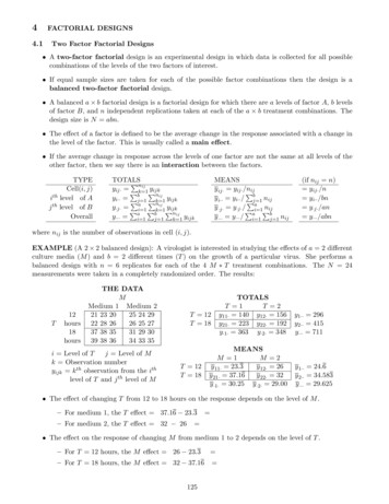
4FACTORIAL DESIGNS4.1Two Factor Factorial Designs A two-factor factorial design is an experimental design in which data is collected for all possiblecombinations of the levels of the two factors of interest. If equal sample sizes are taken for each of the possible factor combinations then the design is abalanced two-factor factorial design. A balanced a b factorial design is a factorial design for which there are a levels of factor A, b levelsof factor B, and n independent replications taken at each of the a b treatment combinations. Thedesign size is N abn. The effect of a factor is defined to be the average change in the response associated with a change inthe level of the factor. This is usually called a main effect. If the average change in response across the levels of one factor are not the same at all levels of theother factor, then we say there is an interaction between the factors.TYPECell(i, j)ith level of Aj th level of BOverallTOTALSPnijyyij· k 1Pb Pijknijyyi·· j 1 k 1Pa Pnij ijky·j· i 1 k 1 yijkP PPnijyijky··· ai 1 bj 1 k 1MEANSy ij· yij· /nijPy i·· yi·· / bj 1 nijPy ·j· y·j· / ai 1 nijPa Pby ··· y··· / i 1 j 1 nij(if nij n) yij· /n yi·· /bn y·j· /an y··· /abnwhere nij is the number of observations in cell (i, j).EXAMPLE (A 2 2 balanced design): A virologist is interested in studying the effects of a 2 differentculture media (M ) and b 2 different times (T ) on the growth of a particular virus. She performs abalanced design with n 6 replicates for each of the 4 M T treatment combinations. The N 24measurements were taken in a completely randomized order. The results:T12hours18hoursTHE DATAMMedium 1 Medium 221 23 2025 24 2922 28 2626 25 2737 38 3531 29 3039 38 3634 33 35i Level of Tj Level of Mk Observation numberyijk k th observation from the ithlevel of T and j th level of MTOTALST 1T 2y11· 140 y12· 156y21· 223 y22· 192y·1· 363 y·2· 348T 12T 18T 12T 18MEANSM 1M 2y 11· 23.3y 12· 26y 21· 37.16y 22· 32y ·1· 30.25 y ·2· 29.00y1·· 296y2·· 415y··· 711y 1·· 24.6y 2·· 34.583y ··· 29.625 The effect of changing T from 12 to 18 hours on the response depends on the level of M .– For medium 1, the T effect 37.16 23.3– For medium 2, the T effect 32 26 The effect on the response of changing M from medium 1 to 2 depends on the level of T .– For T 12 hours, the M effect 26 23.3 – For T 18 hours, the M effect 32 37.16 125

If either of these pairs of estimated effects are significantly different then we say there exists asignificant interaction between factors M and T . For the 2 2 design example:– If 13.83 is significantly different than 6 for the M effects, then we have a significant M Tinteraction.Or,– If 2.6 is significantly different than 5.16 for the T effects, then we have a significant M Tinteraction. There are two ways of defining an interaction between two factors A and B:– If the average change in response between the levels of factor A is not the same at all levels offactor B, then an interaction exists between factors A and B.– The lack of additivity of factors A and B, or the nonparallelism of the mean profiles of A andB, is called the interaction of A and B. When we assume there is no interaction between A and B, we say the effects are additive. An interaction plot or treatment means plot is a graphical tool for checking for potentialinteractions between two factors. To make an interaction plot,1. Calculate the cell means for all a · b combinations of the levels of A and B.2. Plot the cell means against the levels of factor A.3. Connect and label means the same levels of factor B. The roles of A and B can be reversed to make a second interaction plot. Interpretation of the interaction plot:– Parallel lines usually indicate no significant interaction.– Severe lack of parallelism usually indicates a significant interaction.– Moderate lack of parallelism suggests a possible significant interaction may exist. Statistical significance of an interaction effect depends on the magnitude of the M SE :For smal values of the M SE , even small interaction effects (less nonparallelism) may be significant. When an A B interaction is large, the corresponding main effects A and B may have little practicalmeaning. Knowledge of the A B interaction is often more useful than knowledge of the main effect. We usually say that a significant interaction can mask the interpretation of significant main effects.That is, the experimenter must examine the levels of one factor, say A, at fixed levels of the otherfactor to draw conclusions about the main effect of A. It is possible to have a significant interaction between two factors, while the main effects for bothfactors are not significant. This would happen when the interaction plot shows interactions in differentdirections that balance out over one or both factors (such as an X pattern). This type of interaction,however, is uncommon.126

4.2The Interaction Model The interaction model for a two-factor completely randomized design is:yijk where(22)µ is the baseline mean,αi is the ith factor A effect,thβj is the j factor B effect,(αβ)ij is the (i, j)th A B interaction effect,th ijk is the random error of the k observation from the (i, j)th cell.We assume ijk IID N (0, σ 2 ). For now, we will also assume all effects are fixed. If (αβ)ij is removed from (22), we would have the additive model:yijk µ αi βj ijk(23) If we impose the constraintsaXi 1αi bXβj 0j 1aX(αβ)ij 0 for all jandi 1bX(αβ)ij 0 for all i,j 1then the least squares estimates of the model parameters areµb αbi βbj c αβij If we substitute these estimates into (22) we getc eijkyijk µb αbi βbj αβij y ··· (y i·· y ··· ) (y ·j· y ··· ) (y ij· y i·· y ·j· y ··· ) eijkwhere eijk is the k th residual from the treatment (i, j)th cell, and eijk For the 2 2 design,y ··· 29.625y 1· 24.6y 2· 34.586y ·1 30.25 Assuming the constraints in (24),α1α2β1β2αβ11αβ12αβ21αβ22 24.6 29.625 34.583 29.625 30.256 29.625 29.006 29.625 23.3 24.6 30.25 29.625 26 24.6 29.00 29.625 37.16 34.583 30.25 29.625 32 34.583 29.00 29.625 127y ·2 29.00(24)

128

4.3Matrix Forms for the Twoway ANOVAExample: Consider a completely randomized 2 3 factorial design with n 2 replications for each of thesix combinations of the two factors (A and B). The following table summarizes the results:Factor ALevels1211,23,5Factor B Levels234,65,65,74,6 Model: yijk µ αi βj (αβ)ij ijk for i 1, 2 j 1, 2, 3 k 1, 2 and ijk N (0, σ 2 )PP2(ii) 3j 1 βj 0 Assume (i)i 1 αi 0P3P(iii)(iv) 2i 1 (αβ)ij 0 for j 1, 2, 3j 1 (αβ)ij 0 for i 1, 2 Thus, for the main effect constraints, we have α2 α1 and β3 β1 β2 . The interaction effect constraints can be written in terms of just αβ11 and αβ12 :αβ12 αβ22 αβ13 αβ23 Thus, the reduced form of model matrix X requires only 6 columns: µ, α1 , β1 , β2 , αβ11 and αβ12 .µα1111111111111 X β1111111 1 1 1 1 1 1 XX 0 (X 0 X) 1 1 12 Thus, αb2 bα1 0.5c αβc 0αβ22121000001100 1 11100 1 1β2αβ110011 1 10011 1 11100 1 1 1 1001112 0 0 0 0 00 12 0 0 0 00 0 8 4 0 00 0 4 8 0 00 0 0 0 8 40 0 0 0 4 8000001000002 1000 12000002 1000 12αβ120011 1 100 1 111 y Xy 054-6-101-6-3 (X 0 X) 1 X 0 y βb3 βb1 βb2 0.75124656355746 4.5-0.5-1.751-0.750 µbαb1βb1βb2cαβ11cαβc αβc 0.75αβ2111c αβc αβc 0.75αβ131112129c αβc αβc 0.75αβ23111212

Alternate Approach: Keeping 1 a b (a b) Columnsµ X 0001111111000000β21100001100000100000β3 αβ11 αβ12 αβ13 αβ21 αβ22 10-301515-301515-2000-1080-1015-301515-3015 0XX 4-1476-1400000000110000010100000000000110001001 y 0Xy 542430112221310118121086 -45 -45 -20 -20 1 -20 180 -6 -6 -6 -6 -6(X 0 X) 1-45702000-0-10-10-101010-6 -14-1476-4-4-4-610 -10 15 15 -30 -4 -4 -4 -14 -14 76 1246563557460000000 0 1 0(X X) X y 4.5µb b1 -.5 α αb2 .5 b -1.75 β1 βb 2 1 βb 3 .75 c αβ -.75 11 c 0 αβ 12 c .75 αβ 13 c αβ .75 c 21 0 αβ 22 cαβ-.7523130

4.4Notation for an ANOVAaX SSA nb(y i·· y ··· )2 the sum of squares for factor A (df a 1)i 1M SA SSA /(a 1) the mean square for factor A SSB nabX(y ·j· y ··· )2 the sum of squares for factor B (df b 1)j 1M SB SSB /(b 1) the mean square for factor B SSAB na Xba XbXX(y ij· y i·· y ·j· y ··· )2[(y ij· y ··· ) (y i·· y ··· ) (y ·j· y ··· )]2 ni 1 j 1i 1 j 1 the A B interaction sum of squares (df (a 1)(b 1))M SAB SSAB /(a 1)(b 1) the mean square for the A B interaction 2P PP SSE ai 1 bj 1 nk 1 yijk y ij· the error sum of squares (df ab(n 1))M SE SSE /ab(n 1) the mean square error SST a Xb XnX(yijk y ··· )2 the total sum of squares (df abn 1)i 1 j 1 k 1 the total sum of squares is partitioned into components corresponding to the terms in the model:a Xb XnX2(yijk y ··· )abXX2 nb(y i·· y ··· ) na(y ·j· y ··· )2i 1 j 1 k 1i 1 nj 1a XbX2(y ij· y i·· y ·j· y ··· ) i 1 j 1nir XX(yij y i· )2i 1 j 1OR The alternate SS formulas for the balanced two factorial design are:SST a Xb XnX2 yijki 1 j 1 k 1SSAB a Xb2Xyij·i 1 j 1n2y···abnSSA aXy2i··i 1bn2y···abn SSA SSB 2y···abnSSB b2Xy·j·j 1an 2y···abnSSE SST SSA SSB SSAB The alternate SS formulas for the unbalanced two factorial design are:SST nija Xb XX2yijki 1 j 1 k 1SSAB a Xb2Xyij·i 1 j 1where N Pai 1Pbnijj 1 nijy2 ···NSSA Pbj 1 nijy2 ···ni·Ni··i 1 SSA SSB , ni· aXy22y···N, n·j 131SSB b2Xy·j·j 1n·j 2y···NSSE SST SSA SSB SSABPai 1 nij .

Balanced Two-Factor Factorial ANOVA TableSource ofVariationSum ofSquaresd.f.MeanSquareFRatioASSAa 1M SA SSA /(a 1)FA M SA /M SEBSSBb 1M SB SSB /(b 1)FB M SB /M SEA BSSAB(a 1)(b 1)M SAB SSAB /(a 1)(b 1)FA B M SAB /M SEErrorSSEab(n 1)M SE SSE /(ab(n 1))——TotalSStotalabn 1————For the unbalanced case, replace ab(n 1) with N ab for the d.f. for SSE and replace abn 1 with N 1P Pfor the d.f. for SStotal where N ai 1 bj 1 nij .4.5Comments on Interpreting the ANOVA TestH0 : (αβ)11 (αβ)12 · · · (αβ)ab vs. H1 : at least one (αβ)ij 6 (αβ)i0 j 0first.– If this test indicates that there is not a significant interaction, then continue testing the hypotheses for the two main effects:H0 : α1 α2 · · · αa vs.H1 : at least one αi 6 αi0H0 : β1 β2 · · · βb vs.H1 : at least one βj 6 βj 0– If this test indicates that there is a significant interaction, then the interpretation of significantmain effects hypotheses can be masked. To draw conclusions about a main effect, we will fixthe levels of one factor and vary the levels of the other. Using this approach (combined withinteraction plots) we may be able to provide an interpretation of main effects. If we assume the constraints in (24), then the hypotheses can be rewritten as:H0 : (αβ)11 (αβ)12 · · · (αβ)ab 0 vs.4.6H1 : at least one (αβ)ij 6 0H0 : α1 α2 · · · αa 0 vs.H1 : at least one αi 6 0H0 : β1 β2 · · · βb 0 vs.H1 : at least one βj 6 0ANOVA for a 2 2 Factorial Design Example We will now use SAS to analyze the 2 2 factorial design data discussed earlier.MT12hours18hoursMedium 121 23 2022 28 2637 38 3539 38 36132Medium 225 24 2926 25 2731 29 3034 33 35