WIXLIB

Examples: Confirmatory Factor Analysis AndStructural Equation ModelingCHAPTER 5EXAMPLES: CONFIRMATORYFACTOR ANALYSIS ANDSTRUCTURAL EQUATIONMODELINGConfirmatory factor analysis (CFA) is used to study the relationshipsbetween a set of observed variables and a set of continuous latentvariables. When the observed variables are categorical, CFA is alsoreferred to as item response theory (IRT) analysis (Fox, 2010; van derLinden, 2016). CFA with covariates (MIMIC) includes models wherethe relationship between factors and a set of covariates are studied tounderstand measurement invariance and population heterogeneity.These models can include direct effects, that is, the regression of a factorindicator on a covariate in order to study measurement non-invariance.Structural equation modeling (SEM) includes models in whichregressions among the continuous latent variables are estimated (Bollen,1989; Browne & Arminger, 1995; Joreskog & Sorbom, 1979). In all ofthese models, the latent variables are continuous. Observed dependentvariable variables can be continuous, censored, binary, orderedcategorical (ordinal), unordered categorical (nominal), counts, orcombinations of these variable types.CFA is a measurement model. SEM has two parts: a measurementmodel and a structural model. The measurement model for both CFAand SEM is a multivariate regression model that describes therelationships between a set of observed dependent variables and a set ofcontinuous latent variables. The observed dependent variables arereferred to as factor indicators and the continuous latent variables arereferred to as factors. The relationships are described by a set of linearregression equations for continuous factor indicators, a set of censorednormal or censored-inflated normal regression equations for censoredfactor indicators, a set of probit or logistic regression equations forbinary or ordered categorical factor indicators, a set of multinomiallogistic regression equations for unordered categorical factor indicators,55

CHAPTER 5and a set of Poisson or zero-inflated Poisson regression equations forcount factor indicators.The structural model describes three types of relationships in one set ofmultivariate regression equations: the relationships among factors, therelationships among observed variables, and the relationships betweenfactors and observed variables that are not factor indicators. Theserelationships are described by a set of linear regression equations for thefactors that are dependent variables and for continuous observeddependent variables, a set of censored normal or censored-inflatednormal regression equations for censored observed dependent variables,a set of probit or logistic regression equations for binary or orderedcategorical observed dependent variables, a set of multinomial logisticregression equations for unordered categorical observed dependentvariables, and a set of Poisson or zero-inflated Poisson regressionequations for count observed dependent variables.For logisticregression, ordered categorical variables are modeled using theproportional odds specification. Both maximum likelihood and weightedleast squares estimators are available.All CFA, MIMIC and SEM models can be estimated using the followingspecial features: Single or multiple group analysisMissing dataComplex survey dataLatent variable interactions and non-linear factor analysis usingmaximum likelihoodRandom slopesLinear and non-linear parameter constraintsIndirect effects including specific pathsMaximum likelihood estimation for all outcome typesBootstrap standard errors and confidence intervalsWald chi-square test of parameter equalitiesFor continuous, censored with weighted least squares estimation, binary,and ordered categorical (ordinal) outcomes, multiple group analysis isspecified by using the GROUPING option of the VARIABLE commandfor individual data or the NGROUPS option of the DATA command forsummary data. For censored with maximum likelihood estimation,unordered categorical (nominal), and count outcomes, multiple group56

Examples: Confirmatory Factor Analysis AndStructural Equation Modelinganalysis is specified using the KNOWNCLASS option of theVARIABLE command in conjunction with the TYPE MIXTUREoption of the ANALYSIS command. The default is to estimate themodel under missing data theory using all available data. TheLISTWISE option of the DATA command can be used to delete allobservations from the analysis that have missing values on one or moreof the analysis variables. Corrections to the standard errors and chisquare test of model fit that take into account stratification, nonindependence of observations, and unequal probability of selection areobtained by using the TYPE COMPLEX option of the ANALYSIScommand in conjunction with the STRATIFICATION, CLUSTER, ION option is used to select observations for an analysiswhen a subpopulation (domain) is analyzed. Latent variable interactionsare specified by using the symbol of the MODEL command inconjunction with the XWITH option of the MODEL command. Randomslopes are specified by using the symbol of the MODEL command inconjunction with the ON option of the MODEL command. Linear andnon-linear parameter constraints are specified by using the MODELCONSTRAINT command. Indirect effects are specified by using theMODEL INDIRECT command. Maximum likelihood estimation isspecified by using the ESTIMATOR option of the ANALYSIScommand. Bootstrap standard errors are obtained by using theBOOTSTRAP option of the ANALYSIS command.Bootstrapconfidence intervals are obtained by using the BOOTSTRAP option ofthe ANALYSIS command in conjunction with the CINTERVAL optionof the OUTPUT command. The MODEL TEST command is used to testlinear restrictions on the parameters in the MODEL and MODELCONSTRAINT commands using the Wald chi-square test.Graphical displays of observed data and analysis results can be obtainedusing the PLOT command in conjunction with a post-processinggraphics module.The PLOT command provides histograms,scatterplots, plots of individual observed and estimated values, plots ofsample and estimated means and proportions/probabilities, and plots ofitem characteristic curves and information curves. These are availablefor the total sample, by group, by class, and adjusted for covariates. ThePLOT command includes a display showing a set of descriptive statisticsfor each variable. The graphical displays can be edited and exported as aDIB, EMF, or JPEG file. In addition, the data for each graphical displaycan be saved in an external file for use by another graphics program.57

CHAPTER 5Following is the set of CFA examples included in this chapter: 5.1: CFA with continuous factor indicators5.2: CFA with categorical factor indicators5.3: CFA with continuous and categorical factor indicators5.4: CFA with censored and count factor indicators*5.5: Item response theory (IRT) models*5.6: Second-order factor analysis5.7: Non-linear CFA*5.8: CFA with covariates (MIMIC) with continuous factorindicators5.9: Mean structure CFA for continuous factor indicators5.10: Threshold structure CFA for categorical factor indicatorsFollowing is the set of SEM examples included in this chapter: 5.11: SEM with continuous factor indicators5.12: SEM with continuous factor indicators and an indirect effectfor factors5.13: SEM with continuous factor indicators and an interactionbetween two factors*Following is the set of multiple group examples included in this chapter: 585.14: Multiple group CFA with covariates (MIMIC) withcontinuous factor indicators and no mean structure5.15: Multiple group CFA with covariates (MIMIC) withcontinuous factor indicators and a mean structure5.16: Multiple group CFA with covariates (MIMIC) withcategorical factor indicators and a threshold structure5.17: Multiple group CFA with covariates (MIMIC) withcategorical factor indicators and a threshold structure using theTheta parameterization5.18: Two-group twin model for continuous outcomes where factorsrepresent the ACE components5.19: Two-group twin model for categorical outcomes where factorsrepresent the ACE components

Examples: Confirmatory Factor Analysis AndStructural Equation ModelingFollowing is the set of examples included in this chapter that estimatemodels with parameter constraints: 5.20: CFA with parameter constraints5.21: Two-group twin model for continuous outcomes usingparameter constraints5.22: Two-group twin model for categorical outcomes usingparameter constraints5.23: QTL sibling model for a continuous outcome using parameterconstraintsFollowing is the set of exploratory structural equation modeling (ESEM)examples included in this chapter: 5.24: EFA with covariates (MIMIC) with continuous factorindicators and direct effects5.25: SEM with EFA and CFA factors with continuous factorindicators5.26: EFA at two time points with factor loading invariance andcorrelated residuals across time5.27: Multiple-group EFA with continuous factor indicators5.28: EFA with residual variances constrained to be greater thanzero5.29: Bi-factor EFA using ESEM5.30: Bi-factor EFA with two items loading on only the generalfactorFollowing is the set of Bayesian CFA examples included in this chapter: 5.31: Bayesian bi-factor CFA with two items loading on only thegeneral factor and cross-loadings with zero-mean and small-variancepriors5.32: Bayesian MIMIC model with cross-loadings and direct effectswith zero-mean and small-variance priors5.33: Bayesian multiple group model with approximatemeasurement invariance using zero-mean and small-variance priors* Example uses numerical integration in the estimation of the model.This can be computationally demanding depending on the size of theproblem.59

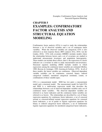
CHAPTER 5EXAMPLE 5.1: CFA WITH CONTINUOUS FACTORINDICATORSTITLE:this is an example of a CFA withcontinuous factor indicatorsDATA:FILE IS ex5.1.dat;VARIABLE: NAMES ARE y1-y6;MODEL:f1 BY y1-y3;f2 BY y4-y6;In this example, the confirmatory factor analysis (CFA) model withcontinuous factor indicators shown in the picture above is estimated.The model has two correlated factors that are each measured by threecontinuous factor indicators.60

Examples: Confirmatory Factor Analysis AndStructural Equation ModelingTITLE:this is an example of a CFA withcontinuous factor indicatorsThe TITLE command is used to provide a title for the analysis. The titleis printed in the output just before the Summary of Analysis.DATA:FILE IS ex5.1.dat;The DATA command is used to provide information about the data setto be analyzed. The FILE option is used to specify the name of the filethat contains the data to be analyzed, ex5.1.dat. Because the data set isin free format, the default, a FORMAT statement is not required.VARIABLE:NAMES ARE y1-y6;The VARIABLE command is used to provide information about thevariables in the data set to be analyzed. The NAMES option is used toassign names to the variables in the data set. The data set in thisexample contains six variables: y1, y2, y3, y4, y5, y6. Note that thehyphen can be used as a convenience feature in order to generate a list ofnames.MODEL:f1 BY y1-y3;f2 BY y4-y6;The MODEL command is used to describe the model to be estimated.Here the two BY statements specify that f1 is measured by y1, y2, andy3, and f2 is measured by y4, y5, and y6. The metric of the factors is setautomatically by the program by fixing the first factor loading in eachBY statement to 1. This option can be overridden. The intercepts andresidual variances of the factor indicators are estimated and the residualsare not correlated as the default. The variances of the factors areestimated as the default. The factors are correlated as the defaultbecause they are independent (exogenous) variables. The defaultestimator for this type of analysis is maximum likelihood. TheESTIMATOR option of the ANALYSIS command can be used to selecta different estimator.61