Transcription
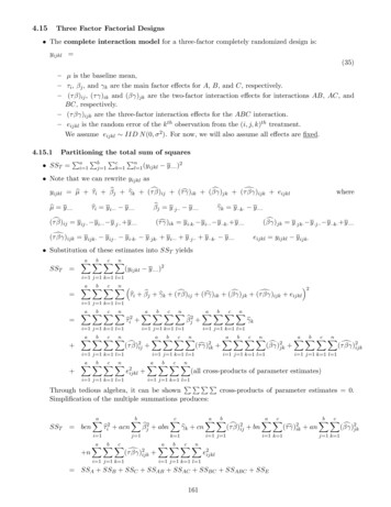
4.15Three Factor Factorial Designs The complete interaction model for a three-factor completely randomized design is:yijkl (35)– µ is the baseline mean,– τi , βj , and γk are the main factor effects for A, B, and C, respectively.– (τ β)ij , (τ γ)ik and (βγ)jk are the two-factor interaction effects for interactions AB, AC, andBC, respectively.– (τ βγ)ijk are the three-factor interaction effects for the ABC interaction.– eijkl is the random error of the k th observation from the (i, j, k)th treatment.We assume eijkl IID N (0, σ 2 ). For now, we will also assume all effects are fixed.4.15.1Partitioning the total sum of squaresP PPP SST ai 1 bj 1 ck 1 nl 1 (yijkl y ···· )2 Note that we can rewrite yijkl asc jk (τdyijkl µb τbi βbj γbk (τcβ)ij (cτ γ)ik (βγ)βγ)ijk eijklτbi y i··· y ····µb y ····βbj y ·j·· y ····(τcβ)ij y ij·· y i··· y ·j·· y ····whereγbk y ··k· y ····(cτ γ)ik y i·k· y i··· y ··k· y ····(τdβγ)ijk y ijk· y ij·· y i·k· y ·jk· y i··· y ·j·· y ··k· y ····c jk y y y y(βγ)·jk··j····k·····eijkl yijkl y ijk· Substitution of these estimates into SST yieldsSST a Xb Xc XnX(yijkl y ···· )2i 1 j 1 k 1 l 1 a Xb Xc Xn Xc jk (τdτbi βbj γbk (τcβ)ij (cτ γ)ik (βγ)βγ)ijk eijkl 2i 1 j 1 k 1 l 1 a Xb Xc XnXτbi2 a Xb Xc XnX(τcβ)2ij i 1 j 1 k 1 l 1 βbj2 i 1 j 1 k 1 l 1i 1 j 1 k 1 l 1 a Xb Xc XnXa Xb Xc XnXa Xb Xc XnX(cτ γ)2ik i 1 j 1 k 1 l 1a Xb Xc XnXe2ijkl i 1 j 1 k 1 l 1γbki 1 j 1 k 1 l 1a Xb Xc XnXa Xb Xc XnXc 2 (βγ)jki 1 j 1 k 1 l 1a Xb Xc XnX(τdβγ)2ijki 1 j 1 k 1 l 1(all cross-products of parameter estimates)i 1 j 1 k 1 l 1PPPPThrough tedious algebra, it can be showncross-products of parameter estimates 0.Simplification of the multiple summations produces:SST bcnaXτbi2 acni 1 na Xb XcXi 1 j 1 k 1bXβbj2 abnj 1(τdβγ)2ijk cXγbk cna XbXi 1 j 1k 1a Xb Xc XnX(τcβ)2ij bna XcXi 1 k 1e2ijkli 1 j 1 k 1 l 1 SSA SSB SSC SSAB SSAC SSBC SSABC SSE161(cτ γ)2ik anb XcXc 2(βγ)jkj 1 k 1
Ii τbiJj βbjc jk(JK)jk βγKk γbk(IJ)ij τcβ ij(IJK)ijk τdβγ ijk(IK)ik τcγ ikEijkl eijkl174162
Three-Factor Factorial Designs: Fixed Factors A, B, CThree Factor Factorial Example In a paper production process, the effects of percentage of hardwood concentration in raw wood pulp,the vat pressure, and the cooking time on the paper strength were studied.175 There were a 3 levels of hardwood concentration (CONC 2%, 4%, 8%).There were b 3 levels of vat pressure (PRESS 400, 500, 650).There were c 2 levels of cooking time (TIME 3 hours, 4 hours).163
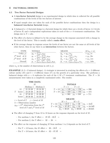
A three factor factorial experiment with n 2 replicates was run. The order of data collection wascompletely randomized. We assume all three factors are fixed. The experimental data are in the table below.HardwoodConcentration246Cooking time 3.0 hoursPressure400500650196.6 197.7199.8196.0 196.0199.4198.5 196.0198.4197.2 196.9197.6197.5 195.6197.4196.6 196.2198.1Cooking time 4.0 hoursPressure400500650198.4 199.6200.6198.6 200.4200.9197.5 198.7199.6198.1 198.0199.0197.6 197.0198.5198.4 197.8199.8 From the SAS output, the p-value .2903 is not significant for the test of the equality of the threefactor interaction effects: H0 : τ βγijk 0 for all i, j, k vs H1 : τ βγijk 6 0 for some i, j, k The p-values of .0843, .0146, and .0750 for the CONC*TIME, CONC*PRESS, and TIME*PRESS twofactor interactions are all significant at the α .10 level indicating the interpretation of the significantmain effects for CONC (p-value .0009), TIME (p-value .0001), and PRESS (p-value .0001) maybe masked. To understand the effects in the model, we need to examine the interaction plots.THREE FACTOR ANALYSIS OF VARIANCEThe GLM ProcedureDependent Variable: strengthSourceDFSum ofSquares Mean Square F Value Pr FModel17 59.728888893.51346405Error180.36555556Corrected Total35 66.308888896.580000009.61 .0001R-Square Coeff Var Root MSE strength Mean0.900767Source0.3052740.604612198.0556DF Type III SS Mean Square F Value Pr Fconc27.763888893.8819444410.620.0009time1 20.2500000020.2500000055.40 2 19.373888899.6869444426.50 ss41.973333330.493333331.350.2903164
199THREE FACTOR ANALYSIS OF VARIANCETHREE FACTOR ANALYSIS OF VARIANCEThe GLM ProcedureThe GLM Procedurestrength198198Distribution of strength197201200200197199strengthDistribution of strength201199strengthstrength199198198THREE FACTOR ANALYSIS OF VARIANCE196196197197The GLM tionof strengthpressLevel ofpressNMeanStd Dev40012 197.5833330.8568794750012 197.4916671.50903843199.0916671.1204368765012Level ofpressN200199strengthLevel ofconcNstrengthMeanStd Dev40012 197.5833330.8568794750012 197.49166765012 199.091667MeanStd Devstrength1.75620113212 198.666667412 197.9583330.9866917512 197.5416671.124486418Level ofconcNMeanStd Dev212 198.6666671.756201131.50903843412 The197.9583330.98669175GLM Procedure1.120436878THREE FACTOR ANALYSIS OF VARIANCE12 197.5416671.12448641THREE FACTOR ANALYSIS OF VARIANCETHREE FACTOR ANALYSIS OF VARIANCEThe GLM ProcedureThe GLM Procedure198Distribution of strength201Distribution of strengthDistribution of h1981991971962 4002 5002 400226505002 65044 400400 4 500198197strengthstrengthconcstrength20188conc1964 5008 400 1988 45006508 6504 6508 4008 5008 65034conc*presstimeconc*pressstrengthLevel of Level ofconcpressNMeanStd DevstrengthLevel oftimeNstrength197MeanStd Dev24004 197.4000001.29614814318 197.3055561.2021902725004 198.4250001.97378655418 198.8055561.12431533650 of 4 200.175000Level of 2 Level44004 197.825000concpressN45004 197.400000248400 4004 198.650000285004 196.6500008650500 6500.69462220Mean0.585235001.19163753Std Dev4 197.4000001961.296148140.736545990.854400374 197.5250000.957427114 198.4250001.008298901.973786554 198.45000026504 200.1750000.6946222044004 197.8250000.5852350045004 197.4000001.1916375346504 198.6500000.8544003784004 197.5250000.73654599Level oftimeN85004 196.6500000.9574271186504 198.4500001.0082989016534timestrengthMeanStd Dev318 197.3055561.20219027418 198.8055561.12431533
199199THREE FACTOR ANALYSIS OF VARIANCEThe GLM ProcedureThe GLM Procedure198strengthTHREE FACTOR ANALYSIS OF VARIANCE198Distribution of stribution of strength2011981961971971963 4003 5001981963 500 3 6503 6503 4004 4004 5004 4004 ength0.875595044006 197.06666735006 196.4000000.766811586 198.4500000.9669539845004650Std Devstrength236 197.5833331.68572437246 199.7500001.061602561.24966662836 196.9000000.9295160046 198.1833336 197.0666670.87559504235006 196.4000000.76681158236506 198.4500000.9669539844006 198.1000000.4560701745006 THREE198.58333346506 199.7333336 199.733333Mean43 of6 197.433333 0.94798031Level of Level446 198.483333 0.76267075conctimeNMean0.45607017MeanStd Dev6 198.1000006 198.5833338384strengthLevel of Level ofconctimeNStd Dev3Level of Level3 of 650400timepress4N3Mean83conc*timestrengthLevel of Level oftimepressN4444conc*timeStd Dev6 197.5833331.6857243746 199.7500001.06160256436 197.4333330.94798031446 198.4833330.762670751.24966662 ANALYSIS86 .9157874640.964192246 198.1833330.96419224The GLM ProcedureDistribution of 350conc*time*pressstrengthLevel of Level of Level ofconctimepressNMeanStd Dev166234002 196.300000 0.4242640780365804408045080465084
SignM0 Pr M 1.0000Signed Rank S Check of Normality-3.5Pr S Assumption0.9570The UNIVARIATE ProcedureVariable: residMomentsTests for NormalityN36 Sum WeightsMeanStd DeviationTest0.1880 Kurtosis-1.1102611StatisticUncorrected SS6.58 Corrected SSWCoeff VariationKolmogorov-Smirnov D0.938963Cramer-von MisesPr W0.0472Pr D 0.01000.07226494Basic Statistical Measures0.172166Variability0.00000 Std Deviationp Value6.58. Std Error -Wilk360 Sum Observations0.43359W-Sq 0.209114 Pr W-Sq 0.0050Median0.00000 Variance0.18800THREE FACTOR ANALYSIS OF VARIANCEMode-0.40000 Range1.70000Interquartile Range 0.75000Anderson-DarlingA-Sq1.090312Prof 4. A-SqNote: The mode displayedis the smallestof 2 modes with a count0.0068The GLM ProcedureTests for Location: Mu0 0TestStatisticp ValueStudent's tt0 Pr t SignM0 Pr M 1.0000Signed Rank S-3.5 Pr S 1.00000.9570Fit Diagnostics for strengthTests for NormalityStatisticShapiro-WilkKolmogorov-Smirnov DRStudent0.0-0.5Pr W0.04720.172166Pr D 0.0100Cramer-von Mises1W-Sq 0.209114 Pr W-Sq 0.0050Anderson-DarlingA-Sq1.090312Pr A-Sq0.0068010-1-1-2-2196 197 198 199 200 201196 197 198 199 200 201Predicted ValuePredicted 5-2-1012Predicted ValueFit–Mean300.100.00196 197 198 199 200 2Percent0.9Leverage2010.5Residual2p Value0.938963Cook's rs18Error DF18MSE0.3656R-Square0.9008Adj R-Square 0.8071010-1-20-1.35-0.450.45Residual1.350.0 0.4 0.80.0 0.4 0.8Proportion Less167301.0
SAS Code for Three-Factor Factorial ** THREE FACTOR ANALYSIS OF VARIANCE ***;*****************************************;DATA in;DO conc 2 , 4 , 8;DO time 3 TO 4;DO press 400 , 500 , 650;DO rep 1 TO 2;INPUT strength @@;strength strength 190;END; END; END; END;CARDS;6.6 6.07.7 6.09.8 9.48.48.5 7.26.0 6.98.4 7.67.57.5 6.65.6 6.27.4 8.17.6OUTPUT;8.68.18.49.6 10.48.7 8.07.0 7.810.6 10.99.6 9.08.5 9.8PROC GLM DATA in PLOTS (ALL);CLASS conc time press;MODEL strength conc time press / SS3;* MEANS press conc time@2;MEANS press conc time;OUTPUT OUT diag R resid;TITLE ’THREE FACTOR ANALYSIS OF VARIANCE’;PROC UNIVARIATE DATA diag NORMAL PLOTS;VAR resid;TITLE "Check of Normality Assumption";RUN;4.16Two Factor Factorial ANOVA with BlocksEXAMPLE: The yield of a chemical process is being studied. The two factors of interest are Temperature and Pressure. Three levels of each factor (a 3, b 3)are selected. Only nine runs can be made in one day. The experimenter runs a complete replicate of the two factorfactorial design on each day. The data are shown in the following table. Analyze the data assuming that the days are blocks. You just have to add a block effect (DAY) to the two factor factorial model.TemperatureLowMediumHigh25086.388.589.1Day 9.491.7Day 2Pressure26085.289.993.227087.390.393.7
TWO-FACTOR FACTORIAL WITH BLOCKSThe GLM ProcedureDependent Variable: yieldSourceSum ofSquares Mean Square F Value Pr FDFModel9 122.8194444Error8Corrected Total13.64660494.250000025.69 .00010.531250017 127.0694444R-Square Coeff Var Root MSE yield Mean0.966554Source0.8208500.72886988.79444DF Type III SS Mean Square F Value Pr Ftemp2 99.85444444press2temp*press4day49.9272222293.98 055562.100.17331 13.0050000013.0050000024.480.0011TWO-FACTOR FACTORIAL WITH BLOCKSThe GLM ProcedureSourceType III Expected Mean SquaretempVar(Error) Q(temp,temp*press)pressVar(Error) Q(press,temp*press)temp*press Var(Error) Q(temp*press)dayVar(Error) 9 Var(day)TWO-FACTORFACTORIAL WITH BLOCKSThe GLM ProcedureTests of Hypotheses for Mixed Model Analysis of VarianceDependent Variable: yieldSourceDF Type III SS Mean SquareF ValuePr F* temp299.85444449.92722293.98 .0001* 11Error: MS(Error)84.2500000.531250* This test assumes one or more other fixed effects are zero.169
yield90yield90TWO-FACTOR FACTORIAL WITH BLOCKSTWO-FACTOR FACTORIAL WITH BLOCKSThe GLM ProcedureThe GLM ProcedureDistribution of yield88Distribution of yield889494928692869090yieldyieldTWO-FACTOR FACTORIAL WITH BLOCKS8888The GLM Procedure8684250868484260 of eld90yieldMeanStd Dev2506 88.51666672.098014932606 88.30000003.44325427Level of270 6pressN89.5666667Level oftempNyield1.74661578yieldL6 85.78333331.11250468MeanStd Dev2506 88.51666672.09801493H6 The91.53333331.74661578GLM Procedure2606 88.30000003.44325427L6 85.78333332706 89.56666672.8380744694MDistributionof yield6 89.06666671.07455417TWO-FACTOR FACTORIAL WITH BLOCKSThe GLM ProcedureThe GLM ProcedureDistribution of yield949292yield90yield9088H 2608488yield9086H 2501.11250468TWO-FACTOR FACTORIAL WITH BLOCKS9284Std Dev6 91.5333333M6 89.0666667 1.07455417Level ofTWO-FACTORFACTORIAL WITH BLOCKStempNMeanStd Dev2.838074469486MeanHDistribution of yield88MMtempyieldLevel ofpressNLtempH 270H 260H 250H 270L 250L 250L 26086LL 260270M25088L 270M 270M 260M 25084M 2601M 270temp*pressyieldLevel of Level oftemppressNHyieldMeanStd DevH2502 90.40000001.83847763H2602 91.70000002.12132034H270Level of Levelof 2 92.5000000L2502 86.2000000temppressNL2602 84.6000000L250MM2702 86.55000002502 88.95000002602 88.6000000Level ofdayNyield86MeanStd Dev19 87.94444442.3016902029 28141.06066017Std Dev2 388291.70000001.83847763HM260H2702 92.50000001.69705627L2502 86.20000000.14142136L2602 84.60000000.84852814L2702 86.55000001.06066017M2502 88.95000000.63639610M2602 88.60000001.83847763M2702 12dayyieldLevel ofdayNMeanStd Dev19 87.94444442.3016902029 89.64444442.99337231
TWO-FACTOR FACTORIAL WITH BLOCKSThe GLM ProcedureFit Diagnostics for 20-1-2-1.0848688909284Predicted yield0.0Cook's D0.5Residual0.7Predicted .092.505Predicted ualTWO-FACTOR FACTORIALWITH BLOCKS30ANALYSIS OF MODEL WITHTWO-FACTORBLOCK INTERACTIONS4220010Observations18Parameters10Error DF8MSE0.5313R-Square0.9666Adj R-Square 0.9289The GLM Procedure-2Dependent Variable: yield-40-1.6 -0.800.81.6SourceResidualDFModel0.0 Sum0.4 0.8of 0.0 0.4 0.8SquaresProportionMeanLess Square F Value Pr F13 126.3861111Error4Corrected Total9.72200850.683333356.910.00070.170833317 127.0694444R-Square Coeff Var Root MSE yield Mean0.994622Source0.4654790.41332088.79444DF Type III SS Mean Square F Value Pr Ftemp2 99.85444444press2temp*press449.92722222292.26 3055566.520.0484FACTORIALWITH BLOCKSdayTWO-FACTOR1 13.0050000013.0050000076.13 0.0010ANALYSIS day*tempOF MODEL WITHTWO-FACTORBLOCKINTERACTIONS2 2.543333331.271666677.44 0.0448day*press21.023333330.51166667TheGLM Procedure3.00SourceType III Expected Mean SquaretempVar(Error) 3 Var(day*temp) Q(temp,temp*press)pressVar(Error) 3 Var(day*press) Q(press,temp*press)0.1603temp*press Var(Error) Q(temp*press)dayVar(Error) 3 Var(day*press) 3 Var(day*temp) 9 Var(day)day*tempVar(Error) 3 Var(day*temp)day*pressVar(Error) 3 Var(day*press)171
TWO-FACTOR FACTORIAL WITH BLOCKSANALYSIS OF MODEL WITH TWO-FACTOR BLOCK INTERACTIONSThe GLM ProcedureTests of Hypotheses for Mixed Model Analysis of VarianceDependent Variable: yieldSourceDF Type III SS Mean Square* tempError: MS(day*temp)299.85444449.92722222.5433331.271667F ValuePr F39.260.0248F ValuePr F5.380.1567* This test assumes one or more other fixed effects are zero.SourceDF Type III SS Mean Square* pressError: MS(day*press)25.5077782.75388921.0233330.511667* This test assumes one or more other fixed effects are zero.SourceDF Type III SS Mean Square F Value Pr .000.1603Error: MS(Error)40.6833330.170833SourcedayErrorDF Type III SS Mean Square F Error: MS(day*temp) MS(day*press) - MS(Error)SAS CodeDM ’LOG; CLEAR; OUT; CLEAR;’;ODS GRAPHICS ON;ODS PRINTER PDF file ’C:\COURSES\ST541\TWOBLOCK.PDF’;OPTIONS NODATE *** TWO-FACTOR FACTORIAL WITH BLOCKS ***;****************************************;DATA in;DO day 1 TO 2;DO temp ’L’ , ’M’ , ’H’;DO press 250 TO 270 BY 10;INPUT yield @@; OUTPUT;END; END; END;CARDS;86.3 84.0 85.8 88.5 87.3 89.0 89.1 90.2 91.386.1 85.2 87.3 89.4 89.9 90.3 91.7 93.2 93.7PROC GLM DATA in PLOTS (ALL);CLASS day temp press;MODEL yield temp press day / SS3;MEANS press temp day;172Pr F0.0728
RANDOM day / TEST;OUTPUT OUT diag P pred R resid;TITLE ’TWO-FACTOR FACTORIAL WITH BLOCKS’;PROC UNIVARIATE DATA diag NORMAL ;VAR resid;*** MODEL INCLUDING BLOCK INTERACTIONS ***;PROC GLM DATA in;CLASS day temp press;MODEL yield temp press day@2 / SS3;RANDOM day day*temp day*press / TEST;TITLE2 ’ANALYSIS OF MODEL WITH TWO-FACTOR BLOCK INTERACTIONS’;RUN;4.17Expected Means Squares (EMS) Algorithm for Balanced Designs (Supplemental) Classify each effect as either a fixed effect or a random effect. A fixed effect is represented by the EMS componentPaPτ2(fixed effect)2For example: i 1 id.f. for the fixed effecta 1 A random effect is represented by a variance component with its associated subscripts. For example:στ2 . An interaction containing at least one random effect is considered random and is represented by avariance component. For example:– If factor A is random and factor B is random, then the A*B interaction is random. Theassociated variance component is στ2β .– If factor A is fixed and factor B is random, then the A*B interaction is random. The associatedvariance component is στ2β .– If factor A is fixed with a levels and factor B is fixed with b levels, then the A*B interaction isPa Pb2i 1 τ βiji 1fixed. The associated EMS component is.(a 1)(b 1)STEP 1: Prepare the EMS Table1. Set up a row for each model effect that has one or more subscripts. Write the error term ij.m as a‘nested’ effect m(ij.) . We say that m(ij.) is the mth replicate for treatment combination ij . . . Wewill use parentheses () to indicate which effects are nested. Nested effects will be discussed in detaillater in the course.2. Set up columns for each subscript. Above each subscript, write the number of levels associated withthe factor and whether the factor is fixed (F) or random (R).3. For each row effect, subscripts are divided into three classes: live, dead, or absent. A subscript is live if it is present and is not in parentheses. A subscript is dead if it is present and is in parentheses. A subscript is absent if it is not present.Example of Step 1: Consider the two-factor factorial design. Factor A is fixed with a levels and factor Bis random with b levels. n replicates were taken for each of the ab combinations of the levels of A and B.We will be using the mixed model yijk µ αi βj αβij ijk .173
Effectαiβjαβij k(ij)FaiComponentP 2αi /(a 1)σβ22σαβσ2RbjRnkEMSSTEP 2: Filling in the rows of the EMS Table:1. Write 1 in each column containing dead subscripts.Effectαiβjαβij k(ij)ComponentP 2αi /(a 1)σβ22σαβσ2FaiRbj11RnkEMS2. If any row subscript corresponds to a random factor (R), then write 1 in all columns with a matchingsubscript. Otherwise, write 0 in all columns with a matching subscript.Effectαiβjαβij k(ij)ComponentP 2αi /(a 1)σβ22σαβσ2Fai011RbjRnk1111EMS3. For the remaining missing values, enter the number of factor levels for that column.Effectαiβjαβij k(ij)ComponentP 2αi /(a 1)σβ22σαβσ2Fai0a11Rbjb111Rnknnn1EMSSTEP 3: Obtaining the EMS1. Consider all rows containing all of the subscripts in the row effect.2. For each row, delete all columns containing live subscripts. Take the product of the remaining valuesand the component.3. EMS the sum of these products.In the example, for αi , there is only one subscript i. In the model αi , αβij , and k(ij) all contain subscripti. We delete the i column and generate the three productsPbn αi22(a)from the αi row(b) nσαβfrom the αβij row(c) σ 2 from the k(ij) row.a 1174
EffectαiComponentP 2αi /(a 1)βjαβij k(ij)σβ22σαβσ2FaiRbjRnk0bna11111nn1EMS2σ 2nσαβPbn αi2 a 1In the example, for βj , there is only one subscript j. In the model βj , αβij , and k(ij) all contain subscriptj. We delete the j column and generate the three products(a) anσβ2 from the βj row,Effect2(b) nσαβfrom the αβij row,αiComponentP 2αi /(a 1)βjαβij k(ij)σβ22σαβσ2(c) σ 2 from the k(ij) row.FaiRbjRnkEMS0bn2σ 2 nσαβ a11111nn12σ 2 nσαβPbn αi2a 1 anσβ2In the example, for αβij , there are two subscripts i and j. In the model αβij and k(ij) all contain subscriptsi and j. We delete the i and j columns and generate the two products2(a) nσαβfrom the αβij rowEffectandαiComponentP 2αi /(a 1)βjαβij k(ij)σβ22σαβσ2(b) σ 2 from the k(ij) row.FaiRbjRnkEMS20bnσ a11111nn1σ2 σ2 2nσαβ2nσαβ2nσαβPbn αi2 a 1 anσβ2Finally, for k(ij) , there are three subscripts i, j, and k. In the model only k(ij) contains all three subscripts.We delete the i, j, and k columns. This leaves only σ 2 .EffectαiComponentP 2αi /(a 1)βjαβij k(ij)σβ22σαβσ2FaiRbjRnkEMS20bnσ a11111nn1σ2 σ2 σ21752nσαβ2nσαβ2nσαβPbn αi2 a 1 anσβ2
Next consider the three-factor factorial design for which all three factors are random. The number of factorlevels are a, b, and c with n replicates taken for each three-factor treatment combination. The full threefactor-factorial model isyijkl µ τi βj γk τ βij τ γik βγjk τ βγijk ijklFrom Step 1 and Step 2, we haveEffectτiβjγkτ βijτ γikβγjkτ βγijk l(ijk)Effectτiβjγkτ βijτ γikβγjkτ βγijk l(ijk)Effectτiβjγkτ βijτ γikβγjkτ βγijk �2στ 2βστ2γ2σβγ2στ 1c11111Rnlnnnnnnn1EMSEMSσ 2 nστ2βγσ 2 nστ2βγσ 2 nστ2βγσ 2 nστ2βγσ 2 nστ2βγσ 2 nστ2βγσ 2 nστ2βγσ2176 bnστ2γ cnστ2β bcnστ22 anσβγ cnστ2β acnσβ22 anσβγ bnστ2γ abnσγ22 cnστ β bnστ2γ2 anσβγ
This is the simplest example when no ratio of EMS exists for defining F -statistics to test certain nullhypotheses. In all of our previous examples, when H0 is trueE(numerator MS) E(denominator MS). For this example, We have exact tests for2 0,(1) H0 : σβγ(2) H0 : στ2γ 0, and(3) H0 : στ2β 0if we use M Sτ βγ as the denominator of the F -statistic. We also have an exact test for(4) H0 : στ2βγ 0 if we use M SE as the denominator of the F -statistic. We do not have exact tests for(5) H0 : στ2 0,(6) H0 : σβ2 0, and(7) H0 : σγ2 0because when (5), (6), or (7) is true, there is no matching EMS. Thus, there is no exact F -test.4.18Approximate F-Tests If we want to make inferences about effects for which there is no exact F -test, we can use approximate F -tests, a procedure attributed to Sattherthwaite (1946). In this procedure, the goal is to find linear combinations of EMS that are equal when H0 is true.That is, findM S 0 M Sr · · · M S sandM S 00 M Su · · · M Svsuch the E(M S 0 ) E(M S 00 ) equals the effect of interest.M S0 The test statistic would be F which is approximately distributed as F (p, q) where the degreesM S 00of freedom p and q arep (M Sr · · · M Ss )2M Sr2 /fr · · · M Ss2 /fsandq (M Su · · · M Sv )2.M Su2 /fu · · · M Sv2 /fvfi is the degrees of freedom associated with mean square M Si . It is unlikely that p and q are integers. Let the A, B, and C be the factors in a three-factor factorial design, and A, B, and C are random.Consider the following:M S 0 M SA M SABCandThen, E(M S 0 ) E(M S 00 ) 177M S 00 M SAB M SAC
Therefore, to test H0 : στ2 0, we can use F p (M SA M SABC )22M SAa 1 M S0with d.f.M S 00and2M SABC(a 1)(b 1)(c 1)q (M SAB M SAC )22M SAB(a 1)(b 1) 2M SAC(a 1)(c 1). Note that when H0 : στ2 0 is true, E(M S 0 ) E(M S 00 ). Note also the choice of M S 0 and M S 00 is not unique. For example, suppose we defineM S 0 M SAM S 00 M SAB M SAC M SABCandThen,E(M S 0 ) E(M S 00 ) σ 2 nστ2βγ bnστ2γ cnστ2β bcnστ2 σ 2 nστ2βγ bnστ2γ cnστ2β bcnστ2 Therefore, to test H0 : στ2 0, we can use F p (M SA )22M SAa 1 a 1andM S0with d.f.M S 00q (M SAB M SAC M SABC )22M SAB(a 1)(b 1) 2M SAC(a 1)(c 1) 2M SABC(a 1)(b 1)(c 1). Again, note that when H0 : στ2 0 is true, E(M S 0 ) E(M S 00 ).4.18.1Determining Exact and Approximate F -tests using SAS Prior to running an experiment that contains random effects, I recommend that you determine whatexact tests and approximate F -tests can be performed. Once you have a design:1. Generate random responses using a random number generator.2. Analyze the random responses in SAS using the RANDOM statement with the /TEST opion.3. Examine the output. For each test of a model effect, see if the denominator of the F -statisticsis a single mean square (exact F -test) or is a linear combination of means squares (approximateF -test). Consider the three factor factorial example and factors A, B, and C are random with a 3, b 2,c 2, and n 3.– There are exact tests for the A B, A C, B C, and A B C effects.– There are only approximate tests for the A, B, and C effects.DATA in;DO A 1 to 3;DO B 1 to 2;DO C 1 to 2;DO rep 1 TO 3;MU A B C;Y MU RANNOR(542057); OUTPUT;END; END; END; END;PROC GLM DATA in;CLASS A B C;MODEL Y A B C / SS3;RANDOM A B C / TEST;TITLE ’THE RANDOM EFFECTS MODEL WITH A, B, AND C RANDOM’;RUN;178
THE RANDOM EFFECTS MODEL WITH A, B, AND C RANDOMThe GLM ProcedureSource Type III Expected Mean SquareAVar(Error) 3 Var(A*B*C) 6 Var(A*C) 6 Var(A*B) 12 Var(A)BVar(Error) 3 Var(A*B*C) 9 Var(B*C) 6 Var(A*B) 18 Var(B)A*BVar(Error) 3 Var(A*B*C) 6 Var(A*B)CVar(Error) 3 Var(A*B*C) 9 Var(B*C) 6 Var(A*C) 18 Var(C)A*CVar(Error) 3 Var(A*B*C) 6 Var(A*C)B*C RANDOMVar(Error) EFFECTS 3 Var(A*B*C) 9 Var(B*C)THEMODELWITH A, B, AND C RANDOMA*B*C Var(Error) 3 Var(A*B*C)The GLM ProcedureTests of Hypotheses for Random Model Analysis of VarianceDependent Variable: YSourceDF Type III SS Mean 78F ValuePr F15.290.6679Error: MS(A*B) MS(A*C) - MS(A*B*C) 22E-17*MS(Error)SourceDF Type III SS Mean F ValuePr F3.990.3872Error: MS(A*B) MS(B*C) - MS(A*B*C) 11E-17*MS(Error)SourceDF Type III SS Mean Square F Value Pr 80.510.6606B*C12.6260132.6260131.640.3287Error: MS(A*B*C)23.2020691.601035SourceDF Type III SS Mean 377F ValuePr F11.570.4048Error: MS(A*C) MS(B*C) - MS(A*B*C) 11E-17*MS(Error)SourceA*B*CError: MS(Error)DF Type III SS Mean Square F Value Pr F23.2020691.6010352416.3618930.6817461792.350.1171
Consider the three factor factorial example and factors A and B are fixed, and factor C is randomwith a 3, b 2, c 2, and n 3.– There are exact tests for the A, B, A B, A C, B C, and A B C effects.– There is an approximate test for the C effect. The ‘Q’ components in the EMS correspond to fixed effects.PROC GLM DATA in;CLASS A B C;MODEL Y A B C / SS3;RANDOM C A*C B*C A*B*C / TEST;TITLE ’THE RANDOM EFFECTS MODEL WITH A, B FIXED AND C RANDOM’;THE RANDOM EFFECTS MODEL WITH A, B FIXED AND C RANDOMThe GLM ProcedureSource Type III Expected Mean SquareAVar(Error) 3 Var(A*B*C) 6 Var(A*C) Q(A,A*B)BVar(Error) 3 Var(A*B*C) 9 Var(B*C) Q(B,A*B)A*BVar(Error) 3 Var(A*B*C) Q(A*B)CVar(Error) 3 Var(A*B*C) 9 Var(B*C) 6 Var(A*C) 18 Var(C)A*CVar(Error) 3 Var(A*B*C) 6 Var(A*C)B*CVar(Error) 3 Var(A*B*C)9 Var(B*C)THE RANDOMEFFECTSMODEL WITHA, B FIXED AND C RANDOMA*B*C Var(Error) 3 Var(A*B*C)The GLM ProcedureTests of Hypotheses for Mixed Model Analysis of VarianceDependent Variable: YSourceDF Type III SS Mean Square* AError: MS(A*C)219.2712079.63560321.6447970.822398F ValuePr F11.720.0786F ValuePr F3.700.3052* This test assumes one or more other fixed effects are zero.SourceDF Type III SS Mean Square* BError: MS(B*C)19.7164439.71644312.6260132.626013* This test assumes one or more other fixed effects are zero.SourceDF Type III SS Mean Square F Value Pr 80.510.6606B*C12.6260132.6260131.640.3287Error: MS(A*B*C)23.2020691.601035SourceDF Type III SS Mean 377F ValuePr F11.570.4048Error: MS(A*C) MS(B*C) - MS(A*B*C) 11E-17*MS(Error)SourceA*B*CError: MS(Error)DF Type III SS Mean Square F Value Pr F23.2020691.6010352416.3618930.6817461802.350.1171
The complete interaction model for a three-factor completely randomized design is: y ijkl (35) { is the baseline mean, { i, j, and k are the main factor e ects for A, B, and C, respectively. { ( ) ij, ( ) ik and ( ) jk are the two-factor interaction e ects for interactions AB, AC, and BC, respectiv