Transcription
SEASONAL TIME SERIES MODELS1
SEASONAL TIME SERIES A time series repeats itself after a regular periodof time. “Business cycle" plays an important role ineconomics. In time series analysis, business cycleis typically represented by a seasonal (orperiodic) model. A smallest time period for this repetitivephenomenon is called a seasonal period, s.2
SEASONAL TIME SERIES3
SEASONAL TIME SERIESSeasonalityStochasticSARIMADeterministic Seasonalmeans(dummies) linear timetrend Sums of cosine curvesat various frequencies linear time trend4
SEASONAL TIME SERIES For deterministic function f(.), we say that f(.) isperiodic with a periodicity s iff t f t k s , k 0, 1, 2, A typical example of a deterministic periodicfunction is a trigonometric series,e.g. sin( ) sin( 2k ) or cos( ) cos( 2k ). The trigonometric series are often used ineconometrics to model time series with strongseasonality. [In some cases, seasonal dummyvariables are used.]5
SEASONAL TIME SERIES For stochastic process Yt, we say that it is aseasonal (or periodic) time series with periodicity sif Yt and Yt ks have the same distribution. For instance, the series of monthly sales of adepartment store in the U.S. tends to peak atDecember and to be periodic with a period 12.OR quarterly ice cream sales is seasonal with period4. In what follows, we shall use s to denoteperiodicity of a seasonal time series. Often s 4and 12 are used for quarterly and monthly timeseries, respectively.6
MODELLING SEASONALITY BY SEASONALDUMMIES One approach to model seasonality isregression on seasonal dummies. It is a simpleapplication of dummy variables defined toreflect movement across the “seasons” of theyear. For quarterly data, s 4, For monthly data, s 12, For weekly data, s 52. For daily data, s 7.7
SEASONAL DUMMY Then we construct s seasonal dummyvariables to indicate the season. So, if we havequarterly data and assuming the firstobservation we have is in the first quarter, wecreate:D1 (1,0,0,0, 1,0,0,0, 1,0,0,0,.)D2 (0,1,0,0, 0,1,0,0, 0,1,0,0, )D3 (0,0,1,0, 0,0,1,0, 0,0,1,0,.)D4 (0,0,0,1, 0,0,0,1, 0,0,0,1,.)8
SEASONAL DUMMY D1 indicates whether we are in the first quarter(i.e., it takes on the value 1 in the first 1 quarterand 0 otherwise), D2 indicates whether we are in the secondquarter, D3 indicates whether we are in the thirdquarter, D4 indicates whether we are in the fourthquarter.9
SEASONAL DUMMY The pure seasonal dummy model is given by:sYt i Dit ti 1 This is simply a regression on an intercept inwhich we allow for a different intercept in eachseason. These different intercepts are called the seasonalfactors and reflect the seasonal pattern over theyear.10
SEASONAL DUMMY If we have s seasons, an alternative is to includejust s-1 seasonal dummies and an intercept. Inthis case:(i) the constant term is the intercept for theomitted season; and(ii) the coefficients on the seasonal dummiesindicate the seasonal increase/decrease relativeto the omitted season. Never include s seasonal dummies and anintercept. This will cause a serious problem.11
SEASONAL DUMMY AND LINEAR TIMETREND If a variable Y exhibits both trend andseasonality, we can combine the trend modelwith the seasonal model and obtain:sYt t i Dit ti 1 Note that since we have used s seasonaldummies, we have dropped the interceptterm from the linear trend part of the model.12
EXAMPLE jj read.table('c:/jj.dat', header FALSE) jj ts(jj, start 1960, frequency 4) 4.751975.751976.751977.751978.751979.751980.7513
EXAMPLELoad FitAR. Write the time series as vector. Look at theBox-Cox results jj.ts as.vector(jj) BoxCox(jj.ts)Use either 0.041-thpower of the seriesor do lntransformationssince the 0.041 isvery close to 0.14
EXAMPLE Q factor(rep(1:4,21))# make (Q)uarter factors [that's repeat 1,2,3,4, 21times] trend time(jj)-1970# not necessary to "center" time, but the results look nicer reg lm(log(jj) 0 trend Q, na.action NULL) # run the regression without anintercept #-- the na.action statement is to retain time series attributes summary(reg)Call:lm(formula log(jj) 0 trend Q, na.action NULL)Residuals:Min1QMedian-0.29318 -0.09062 -0.011803Q0.08460Max0.27644Coefficients:Estimate Std. Error t value Pr( t )trend 0.1671720.00225974.00 2e-16 ***Q11.0527930.02735938.48 2e-16 ***Q21.0809160.02736539.50 2e-16 ***Q31.1510240.02738342.03 2e-16 ***Q40.8822660.02741232.19 2e-16 ***--Signif. codes: 0 ‘***’ 0.001 ‘**’ 0.01 ‘*’ 0.05 ‘.’ 0.1 ‘ ’ 1Residual standard error: 0.1254 on 79 degrees of freedomMultiple R-squared: 0.9935,Adjusted R-squared: 0.9931F-statistic: 2407 on 5 and 79 DF, p-value: 2.2e-1615
EXAMPLE plot(log(jj), type "o")# the data in black with little dots lines(fitted(reg), col 2) # the fitted values in bloody red or use lines(reg fitted, col 2)16
EXAMPLEPlot of the residuals and the ACF of the residuals:17
FORECASTING SEASONAL SERIES The full model is given by:sYt t i Dit ti 1 So, at time t n h, we have:sYn h n h i Di ,n h n hi 1 Note that to construct this forecast we will set n h to its unconditional expectation of zero.18
FORECASTING SEASONAL SERIES To make this point forecast operation wereplace the unknown population parameterswith OLS point estimates:sYˆn h ˆ n h ˆi Di ,n hi 1 Finally, forecasts are formed.19
SEASONALITY Seasonality can reflect other types calendareffects. The “standard” seasonality model with“seasonal dummies” is one type of calendareffect. Two other types of seasonality are holidayvariation and trading-day variation. Holiday variation refers to the fact the dates ofsome holidays change over time. Easter Sunday isan important example, and we may want toinclude in a model with monthly data an “Easterdummy” which equals 1 if the month containsEaster and 0 otherwise.20
SEASONALITY Likewise, trading-day variation refers to the factthat different months contain numbers of tradingor business days. In a model of monthly retailsales, it would certainly seem to matter if therewere, for example, 28, 29, 30, or 31 trading daysin the month. To account for this we couldinclude a trading-day variable which measuresthe number of trading days in the month. We will not focus on holiday and trading-dayvariation effects, even though they are importantin the analysis of many time series.21
PURE SEASONAL TIME SERIES SARIMA(P,D,Q)s P B 1 Bs Y s Dt Q B ts0where 0 is constant, Q B s 1 1B s 2 B 2 s Q B sQ P B s 1 1B s 2 B 2 s P B sP22
SARIMA(0,0,1)12 SMA(1)12 This is a simple seasonal MA model.Yt 0 t t 12 Invertibility: 1. E(Yt) 0. Var Yt 1 22 , k 12 2ACF : k 1 0, o.w.23
SARIMA(1,0,0)12 This is a simple seasonal AR model. 1 B Y 12t0 t Stationarity: 1.E Yt 01 Var Yt 21 2ACF : 12k k , k 0, 1, 2, When 1, the series is non-stationary. To testfor a unit root, consider seasonal unit root tests.24
MULTIPLICATIVE SEASONAL TIME SERIES A special, parsimonious class of seasonal timeseries models that is commonly used inpractice is the multiplicative seasonal modelARIMA(p, d, q)(P,D,Q)s. p B P B 1 B 1 Bsd Y s Dt s B B t0qQwhere all zeros of (B); (Bs); (B) and (Bs)lie outside the unit circle. Of course, there areno common factors between (B) (Bs) and (B) (Bs).25
MULTIPLICATIVE SEASONAL TIME SERIES26
MULTIPLICATIVE SEASONAL TIME SERIES27
MULTIPLICATIVE SEASONAL TIME SERIES28
MULTIPLICATIVE SEASONAL TIMESERIES29
MULTIPLICATIVE SEASONAL TIMESERIES30
Monthly Carbon Dioxide Levels atAlert, NWT, Canada31
AIRLINE MODEL SARIMA(0,1,1)(0,1,1)12 1 B 1 B12 Y 1 B 1 B 12ttwhere 1 and 1. This model is the most used seasonal model inpractice. It was proposed by Box and Jenkins(1976) for modeling the well-known monthlyseries of airline passengers.32
AIRLINE MODEL Let Wt (1 B)(1 B12)Yt, where (1 B) and(1 B12) are usually referred to as the “regular"and “seasonal" difference, respectively.33
AIRLINE MODELWt 1 B 1 B12 tWt t t 1 t 12 t 13Wt I 0 ,k 1 1 2 1 2 2 , k 02 1 22 1 , k 1 , k 12 2 22 1 k 1 , k 12 k 2, k 11,13 , k 11,13221 1 0, o.w. 0, o.w. 34
SEASONAL UNIT ROOTS Seasonal unit roots and testing for seasonalintegration is discussed in Charemza andDeadman (1997, 105-9) and Pfaff (2008). The main advantage of seasonal unit roottests is where you need to make use of datathat cannot be seasonally adjusted or even asa pretest before seasonal adjustment.35
SEASONAL UNIT ROOTS If a series has seasonal unit roots, then standardADF test statistic do not have the same distributionas for non-seasonal series. Furthermore, seasonallyadjusting series which contain seasonal unit rootscan alias the seasonal roots to the zero frequency,so there is a number of reasons why economistsare interested in seasonal unit roots. Hylleberg, S., Engle, R.F., Granger, C. W. J., and Yoo,B. S., Seasonal integration and cointegration,(1990),Journal of Econometrics, 44: pages 215{238.36
THE DICKEY-HASZA-FULLER TEST37
DHF TEST The problem of the DHF test is that, under thenull hypothesis, one has exactly s unit roots.Under the alternative, one has no unit root.This is very restrictive, as some people maywish to test for specific seasonal or nonseasonal unit roots. The HEGY test byHylleberg, Granger, Engle, Yoo can do this.Therefore, it is the most customary test.38
SEASONAL UNIT ROOTS The HEGY test for seasonal integration isconducted by estimating the followingregression (specialcase4 for quarterlydata):4k 4Yt t b j Q jt iWit 1 4Yt tj 2i 1 1where Qjt is a seasonal dummy, and the Wit aregiven below.W1t 1 B 1 B 2 YtW2t 1 B 1 B Yt2W3t 1 B 1 B YtW4t B 1 B 1 B Yt W3t 139
HEGY TEST After OLS estimation, tests are conducted forπ1 0, for π2 0 and a joint test of thehypothesis π3 π4 0. The HEGY test is a joint test for LR (or zerofrequency) unit roots and seasonal unit roots.If none of the πi are equal to zero, then theseries is stationary (both at seasonal andnonseasonal frequencies).40
HEGY TEST Interpretation of the different πi is as follows:1. If π1 0, then there is no long-run(nonseasonal) unit root. π1 is on W1t S(B)Ytwhich has had all of the seasonal rootsremoved.2. If π2 0, then there is no semi-annual unitroot.3. If π3 and π4 0, then there is no unit root inthe annual cycle.41
42
HEGY TEST Just as in the ADF tests, it is important to ensurethat the residuals from estimating the HEGYequation are white noise. Thus, in testing forseasonal unit roots, it is important to follow thesequential procedures detailed above. Again, begin by testing for the appropriate laglength for the dependent variable (to ensureserially uncorrelated residuals), and then testwhether deterministic components belong in themodel.43
HEGY TEST The presence of seasonal unit roots at some frequencyand not at other frequencies can lead to problems ofinterpretation. The presence of a seasonal unit root ata certain frequency implies that there is nodeterministic cycle at that frequency but a stochasticcycle. The power of unit root tests is low, that is, it is not easyto distinguish between genuine unit roots and nearunit roots. The literature suggests that this might notbe too large a problem, as erroneously imposing a unitroot seems better than not imposing it when oneshould.44
OSBORN-CHUI-SMITHBIRCHENHALL (1988) TEST Osborn, Chui, Smith and Birchenhall [1988]test is the modification of Dickey, Hasza andFuller [1984]. In R, seasonal unit root tests are implementedin the CRAN-package forecast package. Osborn et al. [1988] suggested replacing Δsztwith Δsyt as the dependent variable.45
OSBORN-CHUI-SMITHBIRCHENHALL (1988) TEST Incidentally, if h 0, this is equivalent with anADF regression for the seasonal differences;i.e., The lag orders k and h should be determinedsimilarly to the procedures proposed for theADF test.46
OSBORN-CHUI-SMITHBIRCHENHALL (1988) TEST Furthermore, it should be noted thatdeterministic seasonal dummy variables canalso be included in the test regression. Therelevant critical values are provided in Osbornet al. [1988] and are dependent on theinclusion of such deterministic dummyvariables and whether the data have beendemeaned at the seasonal frequency.47
OSBORN-CHUI-SMITHBIRCHENHALL (1988) TEST If the null hypothesis of the existence of a seasonalunit root is rejected for a large enough absolute tratio, then one might conclude that stochasticseasonality is not present or that stochasticseasonality, which can be removed by using sdifferences, does not exist. On the other hand, if thenull hypothesis cannot be rejected, it is commonpractice to consider the order of non-seasonaldifferencing required to achieve stationarity insteadof considering higher orders of seasonal differencing.48
Number of differences requiredfor a stationary series (ndiffs) ndiffs {forecast}ndiffs uses a unit root test to determine the number ofdifferences required for time series x to be made stationary.If test "kpss", the KPSS test is used with the null hypothesisthat x has a stationary root against a unit-root alternative.Then the test returns the least number of differencesrequired to pass the test at the level alpha. If test "adf", theAugmented Dickey-Fuller test is used and if test "pp" thePhillips-Perron test is used. In both of these cases, the nullhypothesis is that x has a unit root against a stationary rootalternative. Then the test returns the least number ofdifferences required to fail the test at the level alpha.49
ndiffs {forecast}nsdiffs uses seasonal unit root tests to determine the number of seasonal differences required fortime series x to be made stationary (possibly with some lag-one differencing as well). If test "ch",the Canova-Hansen (1995) test is used (with null hypothesis of deterministic seasonality) andif test "ocsb", the Osborn-Chui-Smith-Birchenhall (1988) test is used (with null hypothesis that aseasonal unit root exists).ndiffs(x, alpha 0.05, test c("kpss","adf", "pp"), max.d 2)nsdiffs(x, m frequency(x), test c("ocsb","ch"), max.D 1) ndiffs(WWWusage)[1] 1 nsdiffs(log(AirPassengers))[1] 1 ndiffs(diff(log(AirPassengers),12))[1] 150
Example: Austrian industrialproduction Data for log production (without taking first differences) is for1957-2009. AIC and also BIC recommend three additionalaugmenting lags, and we estimate the regression:by OLS. First, we analyze the t–statistics for 1 and 2, and thenthe F–statistic for 3 4 0.51
Example (Contd.) The statistic t( 1) is 2.10. Using the usual Dickey-Fullerμ, we see that this is insignificant. There is evidence ona unit root at 1, as expected. The statistic t( 2) is 2.74. According to HEGY, we revertits sign. The literature gives a critical 5% value at 3.11and a critical 10% value at 2.54 . Because 2.54 2.74 3.11, the unit root at 1 is rejected at 10% butnot at 5%. The statistic F( 3, 4) is 8.08. This is larger than the 5%significance point by HEGY of 6.57, though smaller thanthe 1% point of 8.79 . The unit root pair at i isrejected at the usual 5% level.52
Example (Contd.) No seasonal unit root at i but some evidenceon a unit root at 1 and convincing evidenceon a unit root at 1. The joint F–test F( 2, 3, 4) has a 1% point of 7.63, which is surpassedby the observed value of 8.48. Thus, the jointtest would tend to reject all seasonal unitroots.53
HEGY for monthly series(Lecture Note of Matthieu Stigler) The HEGY test has been extended for monthlyseries (12 roots) by Franses (1990) andBeaulieu and Miron (1993). The roots are the same as HEGY (1,-1, i,-1)plus 1/2(1 31/2 i), 1/2(31/2 i)54
HEGY Test for Monthly Series(Lecture Note of Matthieu Stigler)55
HEGY tests with R (Lecture Note of Matthieu Stigler) The HEGY test and its extension to monthly data ara available in R in: library(uroot) data(AirPassengers) lairp - log(AirPassengers) test - HEGY.test(wts lairp, itsd c(1, 1, c(1:11)), regvar 0, selectlags list(mode "bic", Pmax 12)) test@stats56
STATIONARITY TEST FOR SEASONALSERIES The test developed by Canova and Hansen(1995) takes as the null hypothesis that theseasonal pattern is deterministic. From:The idea is (provided stationarity, i.e. 1 ) totest for instability of the i parameters as theKPSS test does.57
STATIONARITY TEST FOR SEASONALSERIESand test that Var(ut) 0. The null hypothesis in the Canova-Hansen test isrejected in case seasonality of a series is not constant.After seasonal adjustment the Canova-Hansen testtherefore should not reject. Note that having noseasonal pattern at all also implies constantseasonality.58
STATIONARITY TEST FOR SEASONALSERIES Canova-Hansen suggest a Lagrange Multipliertest statistic whose distribution is known asvon Mises distribution. The test is rejected forthe large values of L-statistics. Canova and Hansen use the assumption thatboth the process under investigation and theexplanatory variables in the null regression donot contain any non-stationary behavior at thezero frequency.59
CANOVA-HANSEN TEST IN RDescriptionThis function computes the Canova-Hansen statistic recursively along subsamples of the original data.UsageCH.rectest (wts, type "moving", nsub 48, frec NULL, f0 1, DetTr FALSE, ltrunc NULL,trace list(remain 1, plot 0, elaps 1))Argumentswts a univariate time series object. type a character string indicating how subsamples are selected. See details.nsub the number of observations in each subsample.frec a vector indicating the frequencies to analyse.f0 a 0-1 (No-Yes) vector of length one indicating wether a first lag of the dependent variable is included or not inthe auxiliar regression. See details.DetTr a logical argument. If TRUE a linear trend is included in the auxiliar regression.ltrunc lag truncation parameter for computing the residuals covariance matrix. By default,round(s*(N/100) 0.25), where eqn{s} is the periodicity of the data and N the number of observations.trace a list object indicating if a trace of the iteration progress should be printed. Three levels of information canbe printed: remain, the percentage of the whole procedure that has been completed; plot, a plot of thecomputed statistics; and elaps, how much time the whole procedure has consumed.DetailsElements of frec must be set equal to 0 if the season assigned to this element is not considered and equals to 1for the frequencies to analyse. The position of each frequency in the vector is as follows: c(pi/2, pi) forquarterly series and c(pi/6, pi/3, pi/2, 2pi/3, 5pi/6, pi) for monthly series.Rejection of the null hypothesis implies that the analysed cycles are non-stationary.60
EXAMPLE Quarterly US beer production data from 1975to 1997.61
EXAMPLE (contd.) library(uroot) CH.test(beer)------ - ------ ---Canova & Hansen test------ - ------ ---Null hypothesis: Stationarity.Alternative hypothesis: Unit root.Frequency of the tested cycles: pi/2 , pi ,L-statistic: 0.817Lag truncation parameter: 4Cannot reject H0. Seasonality pattern is deterministic. No seasonalunit rootCritical values:0.10 0.05 0.025 0.010.846 1.01 1.16 1.3562
EXAMPLE (contd.) HEGY.test(wts beer, itsd c(1, 1, c(1:3)), regvar 0,selectlags list(mode "bic", Pmax 12))---- ---HEGY test---- ---Null hypothesis: Unit root.Alternative hypothesis: Stationarity.---HEGY statistics:Stat. p-valuetpi 1 -3.3390.085tpi 2 -5.9440.010Fpi 3:4 13.238 0.010Fpi 2:4 18.546NAFpi 1:4 18.111NAThere is a unit root. The first order differencing is required.No seasonal unit root. Nonseasonal differencing is needed.63
STATIONARITY TEST IN R64
65
DUMMIES One approach to model seasonality is regression on seasonal dummies. It is a simple application of dummy variables defined to reflect movement across the “seasons” of the y