Transcription
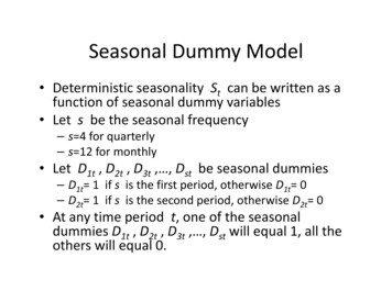
Seasonal Dummy Model Deterministic seasonality St can be written as afunction of seasonal dummy variables Let s be the seasonal frequency– s 4 for quarterly– s 12 for monthly Let D1t , D2t , D3t , , Dst be seasonal dummies– D1t 1 if s is the first period, otherwise D1t 0– D2t 1 if s is the second period, otherwise D2t 0 At any time period t, one of the seasonaldummies D1t , D2t , D3t , , Dst will equal 1, all theothers will equal 0.
Seasonal Dummy Model Deterministic seasonality γ1 γ St 2 M γ 12ifift Januaryt FebruaryMift Decembers γ i Diti 1a linear function of the dummy variables
Estimation Least squares regressionsyt h γ i Dit eti 1s 1 You can either α β i Dit eti 1– Regress y on all the seasonal dummies, omitting the intercept,or– Regress y on an intercept and the seasonal dummies, omittingone dummy (one season, e.g. December) You cannot regress on both the intercept plus all seasonaldummies, for they would be collinear and redundant.
Interpreting Coefficients In the models 1S t α β i Diti 1the intercept α γs is the seasonality in theomitted season. The coefficients βi γi ‐γs are the difference inthe seasonal component from the s’th period.
STATA Programming If the time index is t and is formatted as atime index, you can determine the periodusing the commandsgenerate m month(dofm(t))generate q quarter(dofq(t))for monthly and quarterly data, respectively(See dates and times in STATA Data manual)
Creating Dummies If m is the month (1 for January, 2 for February, etc.), thengenerate m1 (m 1)This creates a dummy variable “m1” for JanuaryThenregress y m1 m2 m3 m4 m5 m6 m7 m8 m9 m10 m11or– regress y m1 m2 m3 m4 m5 m6 m7 m8 m9 m10 m11 m12, noconstant–––– Easier–––––Type “b12.m” in the regressor listregress y b12.mThis includes dummies for months 1 through 11, omits 12Same as mechanically listing the eleven dummies, but easier.It is important that “m” be the numerical month (1 for January, 2 forFebruary, etc.)
Estimation
Estimated Seasonality – Housing 114December96
Housing Starts, by year, and estimatedseasonality
Predicted Values
Example 1Unemployment Rate
Unemployment Rate, by year, andestimated seasonality
Predicted Values
Example 2Gasoline Sales
Gasoline Sales, by year, and estimatedseasonality
Predicted Values
Application – Weekly Data Unemployment Insurance ClaimsDepartment of LaborIssued WeeklyImportant indicator for unemployment
Unemployment ClaimsNot Seasonally Adjusted
Unemployment ClaimsOfficial Seasonally Adjusted Series
Estimation
Estimated Seasonal Process
Seasonally Adjusted(by Dummy Variable Method)
Other types of seasonality Daily data– Day of the week– Handle by including dummy variables for each day High‐frequency data– Include hourly or time‐of‐day indicators Holiday effects– Flower sales big on Valentines Day, Mothers Day, Easter,yet these days can move around– Trading‐day/business‐day variation Number of trading days/business days varies across months Can divide by number of trading days, or include as a regressor
Seasonal Cycle Consider a components model with seasonaland AR(1) cycley t S t CtCt βCt 1 et The seasonal St is a set of seasonal dummiessS t α i Diti 1
Transformationy t S t CtCt βCt 1 et Take the first equation and lag it onceyt 1 St 1 Ct 1 Multiply it by ββyt 1 βSt 1 βCt 1 Then subtract it from the first equation to findyt βyt 1 St βSt 1 et
Seasonal Representation We findyt βyt 1 St βSt 1 et When the seasonal St is a set of seasonaldummies, one for each season, this equationsuggests a regression on– yt‐1– Seasonal dummies– Lagged Seasonal dummies
Redundant But lagged seasonal dummies are redundantwith the original seasonal dummies The set of lagged dummy variables arecollinear with the current dummy variables Given that you know this month is February,there is no information in knowing that lastmonth was January. The lagged dummies can be (should be)omitted
Seasonal Cycle We have found that the regression model issyt α i Dit β yt 1 eti 1ors 1yt α 0 α i Dit β yt 1 eti 1
AR(p) Case If the cycle is an AR(p) we havesyt α i Dit β1 yt 1 L β p yt p eti 1 Estimate by least squares Linear Forecasting
Trend Seasonal Cycle A full model isyt Tt St CtTt μ1 μ 2tsSt α i Diti 1Ct β1Ct 1 L β p Ct p et
Regression Model The implied regression model issyt α i Dit γt β1 yt 1 L β p yt p eti 1 This can be estimated by least‐squares It is a complete forecasting model
Example: NSA Unemployment Rate
Regress on Dummies plus AR(12)
AR Coefficients
Fitted Values
Last 2 years
12‐month forecast
Forecasting with Seasonal Dummy To forecast in STATA with seasonal dummies, thedummy variables must be defined for the forecastperiod After you use the tsappend command, you createthe month variable.gen m month(dofm(t))or.replace m month(dofm(t)) Otherwise m will have missing values for theforecast period
Example: Retail Sales U.S. Census Bureau– Monthly Retail Sales– Not Seasonally Adjusted and Seasonally Adjusted– Sales listed by variety of categories– 1992‐2009
From Census Bureau SpreadsheetJan. 2009Feb. 2009Mar. 2009Apr. 2009May 2009Jun. 2009NOT ADJUSTEDRetail and food services sales, ail sales and food services excl motor vehicle and ail sales, ail sales, total (excl. motor vehicle and parts GAFO(1)83,32382,91887,47787,24893,06988,330Motor vehicle and parts ile and other motor vehicle ile dealers41,79041,63246,83445,37346,60148,405New car ed car dealers5,7586,3286,2595,8815,660Automotive parts, acc., and tire ,53014,54515,36215,519Furniture and home furnishings stores7,4287,2197,6017,2937,6897,728Furniture stores4,2304,2964,2623,9694,2614,148Home furnishings stores3,1982,9233,3393,3243,4283,580Floor covering stores1,3811,3351,4481,4751,4621,673All other home furnishings stores1,6981,4801,7621,7251,8511,790Electronics and appliance stores8,6418,4817,9297,2527,6737,791Appl.,TV, and other elect. stores6,7066,6155,9365,3745,8275,857Household appliance stores1,3061,2011,2491,2521,3171,349Radio, T.V., and other elect. stores5,4005,4144,6874,1224,5104,508Computer and software stores1,7341,7221,7901,6791,6121,706Furniture, home furn, electronics, and appliance stores
Liquor Sales Beer, wine and liquorSample: 1992‐2009Not Seasonally AdjustedBig spike in December
Liquor Sales (Millions of )
ln(Liquor Sales)
Residual from Linear Trend
Seasonal Dummy
Residuals after Seasonal Dummies
Full Estimation
AR Coefficients
Fitted Values
Last 3 years
Residuals
12‐Month Forecast
12‐month forecast The big jump down in the forecast for January2010 is because of the seasonal dummy effect
be seasonal dummies – D 1t 1 if s is the first period, otherwise D 1t 0 – D 2t 1 if s is the second period, otherwise D 2t 0 At any time period t, one of the seasonal dummies D 1t, D 2t
