Transcription
Chapter 11: Computed TomographySlide set of 190 slides based on the chapter authored byJ Gelijnsof the IAEA publication (ISBN 978-92-0-131010-1):Diagnostic Radiology Physics:A Handbook for Teachers and StudentsObjective:To familiarize the student with CT scanning principles, acquisitionand reconstruction, technology and image quality.Slide set preparedby S. EdyveanIAEAInternational Atomic Energy Agency
CHAPTER 11.11.1.11.2.11.3.11.4.11.5.11.6.TABLE OF CONTENTSIntroductionCT principlesThe CT imaging systemImage reconstruction and processingAcquisitionComputed tomography image qualityBibliographyIAEADiagnostic Radiology Physics: a Handbook for Teachers and Students – chapter 11, 2
11.1INTRODUCTIONClinical Computed Tomography (CT) was introduced in1971 - limited to axial imaging of the brain inneuroradiologyIt developed into a versatile 3D whole body imagingmodality for a wide range of applications in for example oncology, vascular radiology, cardiology, traumatology andinterventional radiology.Computed tomography can be used for diagnosis and follow-up studies of patients planning of radiotherapy treatment screening of healthy subpopulations with specific risk factors.IAEADiagnostic Radiology Physics: a Handbook for Teachers and Students – chapter 11, 3
11.1INTRODUCTIONNowadays dedicated CT scanners are available for specialclinical applications, such as For radiotherapy planning - these CT scanners offer an extra widebore, allowing the CT scans to be made with a large field of view. The integration of CT scanners in multi modality imagingapplications, for example by integration of a CT scanner with aPET scanner or a SPECT scanner.IAEADiagnostic Radiology Physics: a Handbook for Teachers and Students – chapter 11, 4
11.1INTRODUCTIONOther new achievements for dedicated diagnostic imagingnew achievements concerns for example the developmentof a dual source CT scanner (a CT scanner that isequipped with two X-ray tubes), and a volumetric CTscanner (a 320 detector row CT scanner that allows forscanning entire organs within one rotation).IAEADiagnostic Radiology Physics: a Handbook for Teachers and Students – chapter 11, 5
11.1INTRODUCTIONCT scanning is perfectly suited for 3D imaging and usedin, for example, brain, cardiac, musculoskeletal, andwhole body CT imagingThe images can be presented as impressive colored 3Drendered images, but radiologists usually rely more onblack and white, 2D images, being either the 2D axialimages, or 2D reformats.IAEADiagnostic Radiology Physics: a Handbook for Teachers and Students – chapter 11, 6
11.2CT PRINCIPLES11.2.1. X-ray projection, attenuation and acquisition oftransmission profilesThe purpose of a computed tomography acquisition is tomeasure x ray transmission through a patient for a largenumber of views.x-ray tubeattenuated beamattenuated beamdetectorelementIAEADiagnostic Radiology Physics: a Handbook for Teachers and Students – chapter 11, 7
11.2CT PRINCIPLES11.2.1. X-ray projection, attenuation and acquisition oftransmission profilesDifferent views are achieved in computed tomographyprimarily by using detectors with hundreds of detector elements along the detectorarc (generally 800-900 detector elements), by rotation of the x ray tube around the patient, taking about 1000angular measurements and by tens or even hundreds of detector rows aligned next toeach other along the axis of rotation 800 – 900detector elements 1000 angularmeasurements1 – 320 detector rowsIAEADiagnostic Radiology Physics: a Handbook for Teachers and Students – chapter 11, 8
11.2CT PRINCIPLES11.2.1. X-ray projection, attenuation and acquisition oftransmission profilesThe values that are assigned to the pixels in a CT imageare associated with the average linear attenuationcoefficient µ (m-1) of the tissue represented within thatpixel.The linear attenuation coefficient (µ) depends on thecomposition of the material, the density of the material,and the photon energy as seen in Beer’s law:I(x) I0 e µx where I(x) is the intensity of the attenuated X ray beam, I0 the unattenuated X ray beam, and x the thickness of the material.I0xµI(x)IAEADiagnostic Radiology Physics: a Handbook for Teachers and Students – chapter 11, 9
11.2CT PRINCIPLES11.2.1. X-ray projection, attenuation and acquisition oftransmission profilesBeer’s law only describes the attenuation of the primarybeam and does not take into account the intensity ofscattered radiation that is generated.For poly-energetic X ray beams Beer’s law should strictlybe integrated over all photon energies in the X rayspectrum.In the back projection methodologies developed for CTreconstruction algorithms, this is generally notimplemented Instead typically a pragmatic solution is to assume where Beer’slaw can be applied using one value representing the averagephoton energy of the X ray spectrum. This assumption causesinaccuracies in the reconstruction and leads to the beam hardeningartefact.IAEADiagnostic Radiology Physics: a Handbook for Teachers and Students – chapter 11, 10
11.2CT PRINCIPLES11.2.1. X-ray projection, attenuation and acquisition oftransmission profilesAs an X ray beam is transmitted through the patient,different tissues are encountered with different linearattenuation coefficients.The intensity of the attenuated X ray beam, transmitted adistance d, can be expressed as:x-ray tubeI0d µ(x)dxI(d) I0 ctor elementIAEADiagnostic Radiology Physics: a Handbook for Teachers and Students – chapter 11, 11
11.2CT PRINCIPLES11.2.1. X-ray projection, attenuation and acquisition oftransmission profilesA CT image is composed of a matrix of pixelsrepresenting the average linear attenuation co-efficientin the associated volume elements (voxels).pixelarrayvoxelIAEADiagnostic Radiology Physics: a Handbook for Teachers and Students – chapter 11, 12
11.2CT PRINCIPLES11.2.1. X-ray projection, attenuation and acquisition oftransmission profilesIllustration: a simplified 4 x 4 matrix representing themeasurement of transmission along one line.Each element in the matrix canin principle have a differentvalue of the associated linearattenuation coefficient.The equation for theattenuation can be expressedas:i 4 I(d) I0 e µi xi 1IAEADiagnostic Radiology Physics: a Handbook for Teachers and Students – chapter 11, 13
11.2CT PRINCIPLES11.2.1. X-ray projection, attenuation and acquisition oftransmission profilesFrom the above it can be seen that the basic data neededfor CT is the intensity of the attenuated and unattenuatedX ray beam, respectively I(d) and I0, and that this can bemeasured.Image reconstruction techniques can then be applied toderive the matrix of linear attenuation coefficients, which isthe basis of the CT image.IAEADiagnostic Radiology Physics: a Handbook for Teachers and Students – chapter 11, 14
11.2CT PRINCIPLES11.2.2. Hounsfield UnitsIn CT the matrix of reconstructed linear attenuationcoefficients (µmaterial) is transformed into a correspondingmatrix of Hounsfield units (HUmaterial), where the HU scaleis expressed relative to the linear attenuation coefficient ofwater at room temperature (µwater):HUmaterial µmaterial µwater 1000µwaterIt can be seen that HUwater 0 as (µmaterial µwater), HUair -1000 as (µmaterial 0) HU 1 is associated with 0.1% of the linear attenuation coefficientof water.IAEADiagnostic Radiology Physics: a Handbook for Teachers and Students – chapter 11, 15
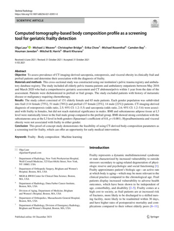
11.2CT PRINCIPLES11.2.2. Hounsfield UnitsTypical values for body tissues. The actual value of the Hounsfield unit depends on thecomposition of the tissue or material, the tube voltage, and thetemperature.SubstanceHounsfield unit (HU)Compact bone 1000 ( 300 to 2500)Liver 60 ( 50 to 70)Blood 55 ( 50 to 60)Kidneys 30 ( 20 to 40)Muscle 25 ( 10 to 40)Brain, grey matter 35 ( 30 to 40)Brain, white matter 25 ( 20 to 30)Water0Fat- 90 (-100 to -80)Lung- 750 (-950 to -600)Air- 1000IAEADiagnostic Radiology Physics: a Handbook for Teachers and Students – chapter 11, 16
CT number windowHounsfield units are usually visualized in an eight bit greyscale offering only 128 grey values.The display is defined using4000 HU4000 HU Window level (WL) as CT number ofmid-grey Window width (WW) as the numberof HU from black - whiteWLWW0 HU0 HUWL-1000 HUWW-1000 HUIAEADiagnostic Radiology Physics: a Handbook for Teachers and Students – chapter 11, 17
11.2CT PRINCIPLES11.2.2. Hounsfield UnitsThe choice of WW and WL is dictated by clinical needOptimal visualization of the tissues of interest in the CTimage can only be achieved by selecting the mostappropriate window width and window level.Different settings of the WW and WL are used to visualizefor example soft tissue, lung tissue or bone.IAEADiagnostic Radiology Physics: a Handbook for Teachers and Students – chapter 11, 18
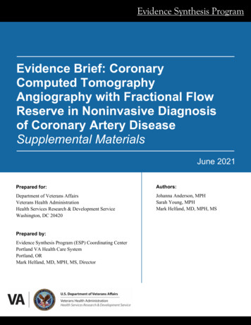
11.2CT PRINCIPLES11.2.2. Hounsfield UnitsSame image data at different WL and WW4000 HU4000 HU0 HUWLWLWWWW-1000 HU-1000 HUWL -593, WW 529WL -12, WW 400GSTT Nuclear Medicine 06IAEADiagnostic Radiology Physics: a Handbook for Teachers and Students – chapter 11, 19
11.2CT PRINCIPLES11.2.2. Hounsfield UnitsThe minimum bit depth that should be assigned to theHounsfield unit is 12, this enables creating a Hounsfieldscale that runs from –1024 HU to 3071 HU, thus coveringmost clinically relevant tissues.A wider Hounsfield scale with a bit depth of 14 is usefulfor extending the Hounsfield unit scale upwards to 15359HU thus making it compatible with materials that have ahigh density and high linear attenuation coefficient.An extended Hounsfield scale allows for bettervisualisation of body parts with implanted metal objectssuch as stents, orthopaedic prosthesis’s, dental- orcochlear implants.IAEADiagnostic Radiology Physics: a Handbook for Teachers and Students – chapter 11, 20
11.2CT PRINCIPLES11.2.2. Hounsfield UnitsFrom the definition of the Hounsfield unit for substances and tissues, except for water and air, variations ofthe Hounsfield units occur when they are derived at different tubevoltages.The reason is that as a function of photon energy differentsubstances and tissues exhibit a non linear relationship oftheir linear attenuation coefficient relative to water.This effect is most notable for substances and tissues thathave a relatively high (effective) atom number such ascontrast enhanced blood (iodine) and bone (calcium).IAEADiagnostic Radiology Physics: a Handbook for Teachers and Students – chapter 11, 21
11.2CT PRINCIPLES11.2.2. Hounsfield UnitsIn clinical practice, considerable deviations between theexpected and the actually observed Hounsfield unit mayoccur.Causes for such inaccuracies may be the dependence ofthe Hounsfield unit for example on the reconstruction filter,on the size of the scanned field of view, and on theposition within the scanned field of view.In addition, image artefacts may have an effect on theaccuracy of the Hounsfield units.IAEADiagnostic Radiology Physics: a Handbook for Teachers and Students – chapter 11, 22
11.2CT PRINCIPLES11.2.2. Hounsfield UnitsWhen performing clinical studies over time, one shouldtake into account that even on the same scanner, withtime, a certain drift of the Hounsfield units may occur.In multicenter studies that involve different CT scanners,significant variations in the observed Hounsfield units mayalso occur between centers.Therefore, quantitative imaging in computed tomographyrequires special attention and often additional calibrationsof the CT scanners are needed.IAEADiagnostic Radiology Physics: a Handbook for Teachers and Students – chapter 11, 23
11.3THE CT IMAGING SYSTEM11.3.1 Historical and current acquisition configurationsAfter the pre-clinical research and development during theearly 1970’s, CT developed rapidly as an indispensableimaging modality in diagnostic radiology.Most of the modern CT technology that is being used inclinical practice nowadays was already described at theend of the year 1983.IAEADiagnostic Radiology Physics: a Handbook for Teachers and Students – chapter 11, 24
11.3THE CT IMAGING SYSTEM11.3.1 Historical and current acquisition configurationsThe development of multi detector-row CT and multisource CT was described in a 1980 United States patent “the figure is a simplified plan view M in which three X-ray sourcesare employed in conjunction with three corresponding rotating Xray detectors”. #4196352, W.H. Berninger, R.W. Redington, GE company.IAEADiagnostic Radiology Physics: a Handbook for Teachers and Students – chapter 11, 25
11.3THE CT IMAGING SYSTEM11.3.1 Historical and current acquisition configurationsThe acquisition technique of helical CT was described in aPatent in 1983 . “the figure is an illustrative representation for explaining thehelically-scanning methodM.by continuous transportation of thetable-couch” #4630202, Issei Mori, Tochigi, Japan.IAEADiagnostic Radiology Physics: a Handbook for Teachers and Students – chapter 11, 26
11.3THE CT IMAGING SYSTEM11.3.1 Historical and current acquisition configurationsCurrently most scanners are helical, multi detector row CTscannersThe technologies of dual source and volumetric CTscanning have however also been implemented on a widescale.Fan beamImPACTz-axisImPACTIAEADiagnostic Radiology Physics: a Handbook for Teachers and Students – chapter 11, 27
11.3THE CT IMAGING SYSTEM11.3.1 Historical and current acquisition configurationsTechnological advances, 1985 - 2007Slip ringscanning,1 s scanDual-slicescanning0.5 secondscanningSixtyEight slice fourscanning slice320row85 86 87 88 89 90 91 92 93 94 95 96 97 98 99 00 01 02 03 04 05 06 07HelicalscanningSub secondscanningFour-slicescanningSixteen Dual X-raysourcesliceImPACTIAEADiagnostic Radiology Physics: a Handbook for Teachers and Students – chapter 11, 28
11.3THE CT IMAGING SYSTEM11.3.2 Gantry and tableThe CT gantry contains all devices that are required torecord transmission profiles of a patient, sincetransmission profiles have to be recorded under differentangles these devices are mounted on a support that canbe rotated.IAEADiagnostic Radiology Physics: a Handbook for Teachers and Students – chapter 11, 29
11.3THE CT IMAGING SYSTEM11.3.2 Gantry and tableOn the rotating part of the gantry are mounted for example the X-ray tube, the detector, the high voltage generator for the Xray tube, the (water or air) cooling of the X-ray tube, the dataacquisition system, the collimator, and the beam shaping filters.DRTTX-ray tubeDX-ray detectorsXX-ray beamRGantry rotationIAEAXCt-internals.jpg commons.wikimediaDiagnostic Radiology Physics: a Handbook for Teachers and Students – chapter 11, 30
11.3THE CT IMAGING SYSTEM11.3.2 Gantry and tableElectrical power is generallyrotating gantry – with tubesupplied to the rotatingand detectorscontactgantry through contactsbrushes(brushes) from stationaryslip rings.powerProjection profiles aretransmitted from the gantryto a computer usually bywireless communication (orcomputerslip ring ic Radiology Physics: a Handbook for Teachers and Students – chapter 11, 31
11.3THE CT IMAGING SYSTEM11.3.2 Gantry and tableThe position of the patient on the table can be head first or feet first supine or proneThe position is usually recorded with the scan data.impactscan.orgIAEADiagnostic Radiology Physics: a Handbook for Teachers and Students – chapter 11, 32
11.3THE CT IMAGING SYSTEM11.3.3 The X-ray tube and generatorAn x ray tube (with a rotating tungsten anode) and highvoltage generator are used for generating the x ray beam.The beam is collimated to create the ‘dose slice’ (or’cone’)High Voltage 70 - 140 kVTube housing-AnodeFilamentElectron beamRotorStatorThin window VacuumtubeMovable Collimator: 1 – 160 mm depending on the scannerZ-axis (patient axis)X-ray beamImPACTIAEADiagnostic Radiology Physics: a Handbook for Teachers and Students – chapter 11, 33
11.3THE CT IMAGING SYSTEM11.3.3 The X-ray tube and generatorRotation time, and the associated temporal resolution ofCT scan, is limited due to the strong increase of centrifugalforces at shorter rotation times.In fast CT scanners with rotation times in the order ofmagnitude of 0.35 seconds, rotating parts are exposed toseveral tenths of g forces.IAEADiagnostic Radiology Physics: a Handbook for Teachers and Students – chapter 11, 34
11.3THE CT IMAGING SYSTEM11.3.4 Collimation and filtrationThe X-ray beam is often referred to as a fan beam wherethe beam width along the longitudinal axis is smallFor multi-slice scanners where the longitudinal beam widthis no longer small the X-ray beam is often referred to as‘cone beam’Side viewapproximates toparallel sides ofbeam for narrowbeam scannersFan beamIAEAx-y plane‘cone beam’ forwider beam multislice scannersz-axisz-axisDiagnostic Radiology Physics: a Handbook for Teachers and Students – chapter 11, 35
11.3THE CT IMAGING SYSTEM11.3.4 Collimation and filtrationBeam shaping filters are being used to create a gradient inthe intensity of the X-ray beam They are sometimes called “bow-tie” filters They are mounted close to the X-ray tube.The purpose of the beam shaping filter is to reduce the dynamic range of the signal recorded by the CTdetector Reduce the dose to the periphery of the patient Attempt to normalise the beam hardening of the beam – to aid withcalibrationIAEADiagnostic Radiology Physics: a Handbook for Teachers and Students – chapter 11, 36
11.3THE CT IMAGING SYSTEM11.3.4 Collimation and filtrationSchematic figure showing the fan beam, flat and beamshaping (‘bow-tie’) filtersx-ray tubeflat filter‘bow-tie’ filterX-ray fan beamdetectorsIAEAImPACTDiagnostic Radiology Physics: a Handbook for Teachers and Students – chapter 11, 37
11.3THE CT IMAGING SYSTEM11.3.5 DetectorsCT scanner detectors 800-1000 detector elements along the detector arc 1 – 320 detectors along z-axisCT detectors are curved in the axial plane (x-y plane), andrectangular along the longitudinal axis (z-axis)outerdetectorsused forcalibrationIAEAx-y planez-axisDiagnostic Radiology Physics: a Handbook for Teachers and Students – chapter 11, 38
11.3THE CT IMAGING SYSTEM11.3.5 DetectorsXenon filled ionization chambers were used till year 2000 Fewer ring artefacts Lower detection efficiencyCurrently solid state detectors are used better detection efficiencyDetector TypeEfficiencyXenon gas filled70%Solid stateApproaching 100%IAEADiagnostic Radiology Physics: a Handbook for Teachers and Students – chapter 11, 39
11.3THE CT IMAGING SYSTEM11.3.5 DetectorsSolid state detectors are generally scintillators the photons interact with the detector and generate light.The light is converted into an electrical signal by photodiodesAn anti-scatter grid may be usedX-raysepta between detectors toprevent photons crossing toneighbouring detectorsvisiblephotonscintillator detectorsphoto-diodeanti-scatter gridImPACTelectrical signalIAEADiagnostic Radiology Physics: a Handbook for Teachers and Students – chapter 11, 40
11.3THE CT IMAGING SYSTEM11.3.5 DetectorsEssential physical characteristics of the CT detectors are Good detection efficiency Fast response (and little afterglow) Good transparency for the generated light (to ensure optimaldetection of the generated light by the photodiodes).IAEADiagnostic Radiology Physics: a Handbook for Teachers and Students – chapter 11, 41
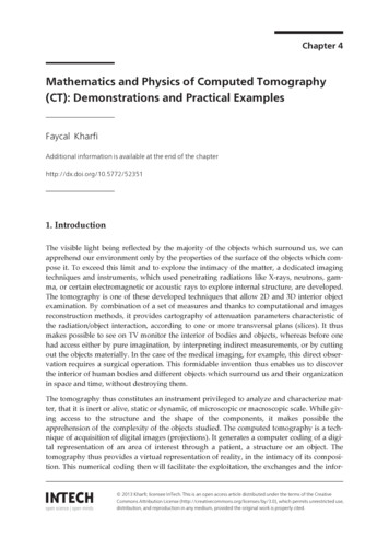
11.3THE CT IMAGING SYSTEM11.3.5 DetectorsThe septa and the strips of the anti scatter grid should beas small as possible, since they reduce the effective areaof the detector and thus reduce the detection of X-rays.Detector modules for a 4, 16, 64 and 320 slice CT scanner (left), thecomplete CT detector is composed of many detector modules (right)(Courtesy Toshiba Medical Systems)IAEADiagnostic Radiology Physics: a Handbook for Teachers and Students – chapter 11, 42
11.3THE CT IMAGING SYSTEM11.3.5 DetectorsResolution in the reconstructed images depends on The size of detector elements - along the detector arc and the z-axis The angular separation of the projectionx-y planez-axisx-y planeImPACTIAEADiagnostic Radiology Physics: a Handbook for Teachers and Students – chapter 11, 43
11.3 THE CT IMAGING SYSTEM11.3.5 DetectorsDetector sizes are the effective size at the iso-centreThe minimum number of detector elementsshould be approximately (2 FOV)/d toachieve a spatial resolution of d in thereconstructed imagex-y plane 800 detector elements are required to achieve aspatial resolution of 1 mm within a reconstructedimage at a field of view of 400 mmdFOVSpatial resolution can be improved by use ofthe quarter detector shiftIt can also be improved by the use of adynamic focal spotSchematic view of detector sizesImPACTIAEADiagnostic Radiology Physics: a Handbook for Teachers and Students – chapter 11, 44
11.3THE CT IMAGING SYSTEM11.3.5 DetectorsQuarter detector shift By shifting the detector elements by a distance of a quarter of thesize of the detector elements, the theoretical achievable spatialresolution becomes twice as good. It is generally implemented in detectors of all CT scanners.no ¼ shiftwith ¼ shiftSchematic view of quarter detector shift – X-Y planeImPACTIAEADiagnostic Radiology Physics: a Handbook for Teachers and Students – chapter 11, 45
11.3THE CT IMAGING SYSTEM11.3.5 DetectorsDynamic or flying focal spot Focal spot position on anode is rapidly oscillated during gantryrotation, doubling the number of projectionsSchematic view of dynamic focal spot – X-Y planeImPACTIAEADiagnostic Radiology Physics: a Handbook for Teachers and Students – chapter 11, 46
11.3THE CT IMAGING SYSTEM11.3.5 DetectorsWith the current detector rows and/or quarter detector shiftand/or flying focal spot a spatial resolution of 0.6 – 0.9mm in the axial plane can be achieved 0.6 – 0.9 mmx-y planeIAEADiagnostic Radiology Physics: a Handbook for Teachers and Students – chapter 11, 47
11.3THE CT IMAGING SYSTEM11.3.5 DetectorsAlong the z-axis multiple detector row scanners givegreater coverage along the patient and allows for shorterscan times and thinner reconstructed slices.The number of rows do not necessarily match the numberof ‘slices of data’ – particularly with early multi-slice CT 4 active detector rows- 199816 active detector rows - 200164 active detector rows in - 2004320 active detector rows - 2007z-axisIAEADiagnostic Radiology Physics: a Handbook for Teachers and Students – chapter 11, 48
11.3THE CT IMAGING SYSTEM11.3.5 DetectorsIncreased coverage of the multi detector row CT scannersincreased with more active detector rowsIAEADiagnostic Radiology Physics: a Handbook for Teachers and Students – chapter 11, 49
11.3THE CT IMAGING SYSTEM11.3.5 DetectorsA multi-slice scanner may be defined by the number of‘data slices’ it acquires – or by the number of detector rows e.g.GE LightSpeed, four slice scanner has 16x 1.25 mm detectors it can acquire 4 x 1.25 mm, 4 x 2.5 mm, 4 x 3.75 mm, or 4 x 5 mm slicesz-axis4 x 1.25 mm4 x 2.5 mm4 x 5 mmImPACTIAEADiagnostic Radiology Physics: a Handbook for Teachers and Students – chapter 11, 50
11.3THE CT IMAGING SYSTEM11.3.5 DetectorsMulti-slice or multi-row scanners enabled Thinner slices Longer scan volumes Faster scan volumesA typical acquisition with a single detector row scannercovered 5 mm.CT scanners with 4 active detector rows achieved asubstantial improvement of the longitudinal resolution. For example, by using 4 active detector rows in a 4 x 1 mmacquisition configuration, the longitudinal spatial resolutionimproved from 5 mm to 1 mmIAEADiagnostic Radiology Physics: a Handbook for Teachers and Students – chapter 11, 51
11.3THE CT IMAGING SYSTEM11.3.5 DetectorsIn clinical practice the CT scanners with 4 active detectorrows were primarily used to enhance longitudinalresolutionThe CT scanners with 4 active detector rows could also beused for enhanced longitudinal coverage, for example byselecting a 4 x 2 8 mm, or even a 4 x 4 16 mmcoverage.Enhanced longitudinal coverage would allow for shorterscan times but without the benefit of improved longitudinalresolution.IAEADiagnostic Radiology Physics: a Handbook for Teachers and Students – chapter 11, 52
11.3THE CT IMAGING SYSTEM11.3.5 DetectorsThe CT scanners with 16 or 64 active detector rowsallowed for acquisitions in for example 16 x 0.5 8 mmand 64 x 0.5 32 mm configurations. These scanners provided excellent longitudinal spatial resolution,high quality 3D reconstructions, and at the same time reducedscan times.The CT scanners with up to 64 active detector rowsgenerally cover a scan volume with a helical acquisitionwith multiple rotations.The 320 detector row CT scanner covers 160 mm on onerotation, for organs such as the brain or the heart within one rotation.IAEADiagnostic Radiology Physics: a Handbook for Teachers and Students – chapter 11, 53
11.4IMAGE RECONSTRUCTION AND PROCESSING11.4.1 General conceptsTechniques for reconstruction include Simple backprojectionAlgebraic reconstructionIterative reconstructionFiltered back projectionIAEADiagnostic Radiology Physics: a Handbook for Teachers and Students – chapter 11, 54
11.4IMAGE RECONSTRUCTION AND PROCESSING11.4.1 General conceptsDuring a CT scan, numerous measurements of thetransmission of X-rays through a patient are acquired atmany anglesThis is the basis for reconstruction of the CT image.x-ray tubeI0attenuationI(d)detector elementx-y planeIAEAImPACTDiagnostic Radiology Physics: a Handbook for Teachers and Students – chapter 11, 55
11.4IMAGE RECONSTRUCTION AND PROCESSING11.4.1 General conceptsThe logarithm of the (inverse) measured normalizedtransmission, ln(I0/I(d)), yields a linear relationship with theproducts of µi x.x-ray tubeI0attenuationi n attenuationdetectorelementI(d)I(d) I0 e µi xi 1µ i x ln(I 0 /I(d))detector positionIAEADiagnostic Radiology Physics: a Handbook for Teachers and Students – chapter 11, 56
11.4IMAGE RECONSTRUCTION AND PROCESSING11.4.1 General conceptsThe figure below shows(a) the X-ray projection under a certain angle(b) leading to one transmission profileThe backprojection distributes the measured signal evenlyover the area(c) under the same angle as the projectionIAEADiagnostic Radiology Physics: a Handbook for Teachers and Students – chapter 11, 57
11.4IMAGE RECONSTRUCTION AND PROCESSING11.4.1 General conceptsTransmission profiles are taken from a large number ofangles and backprojected(d) yielding a strongly blurred imageMathematics shows that simple backprojection is notsufficient for accurate image reconstruction in CT.Instead a filtered backprojection must be used It is the standard for image reconstruction in CT.IAEADiagnostic Radiology Physics: a Handbook for Teachers and Students – chapter 11, 58
11.4IMAGE RECONSTRUCTION AND PROCESSING11.4.1 General conceptsOther reconstruction techniques are algebraic or iterativereconstructions.Algebraic reconstruction solves a number of simultaneousequations.For example Projections in two horizontal, twovertical, and two diagonal directionsyield six projection values. These values can be used to solvean overcomplete set of six equations. The equations can be solvedand they yield the 2 x 2 image matrix.IAEADiagnostic Radiology Physics: a Handbook for Teachers and Students – chapter 11, 59
11.4IMAGE RECONSTRUCTION AND PROCESSING11.4.1 General conceptsAlgebraic reconstruction in clinical practice is not feasible, due to the large (512 x 512) matrices that are used in medicalimaging due to inconsistencies in the equations due to measurement errorsand noise.IAEADiagnostic Radiology Physics: a Handbook for Teachers and Students – chapter 11, 60
11.4IMAGE RECONSTRUCTION AND PROCESSING11.4.1 General conceptsIterative (statistical) reconstructions are sometimes used These are routinely used in nuclear medicine. They are becoming available for commercial CT scannersPotential benefits of iterative reconstructions the removal of streak artefacts (particularly when fewer projectionangles are used) better performance in low-dose CT acquisitionsHowever, images may be affected by other artefacts aliasing patterns overshoot in the areas of sharp intensity transitionsIAEADiagnostic Radiology Physics: a Handbook for Teachers and Students – chapter 11, 61
11.4IMAGE RECONSTRUCTION AND PROCESSING11.4.2 Object, image and radon spaceFiltered backprojection is the most frequently appliedtechnique for CT reconstructionTo understand this it is essential to introduce threeinterrelated domains: Object space, Radon space, Fourier space.The three spatial domains are interrelated, and theirrelationships can be described mathematically.IAEADiagnostic Radiology Physics: a Handbook for Teachers and Students – chapter 11, 62
11.4IMAGE RECONSTRUCTION AND PROCESSING11.4.2 Object, image and radon spaceThe three domains associated with the technique offiltered backprojection area) Object space (linear attenuation values),b) Radon space (projection values recorded under many angles) this domain is also referred to as sinogram space where Cartesian coordinatesare used),c) Fourier space which can be derived from object space by a 2D Fourier transform.(a)(b)Object space(c)Radon spaceFourier spaceIAEADiagnostic Radiology Physics: a Handbook for Teachers and Students – chapter 11, 63
11.4IMAGE RECONSTRUCTION AND PROCESSING11.4.2 Object, image and radon spaceThe figure below illustrates the interrelations between thethree domains for one projection angle.(a) One specific projection angle in object space(b) The projection that is recorded by the CT scanner(c) This projection corresponds with one line in Radon space(d) One angulated line in Fourier space is created from a 1-Dtransform of the recorded line in the sinogram1-D FTObject spaceRadon spaceFourier spaceIAEADia
Clinical Computed Tomography (CT) was introduced in 1971 -limited to axial imaging of the brain in neuroradiology It developed into a versatile 3D whole body imaging modality for a wide range of applications in for example oncology, vascular radiology, cardiology, traumatology and interventional radiol