WIXLIB

86Imaging and Radioanalytical Techniques in Interdisciplinary Research - Fundamentals and Cutting Edge ApplicationsBefore continuing our mathematical development and demonstration specific to the objectscanning in transmission tomography, it is useful to give some math reminder on Radontransform and its main properties.Math Reminder 1.The Radon transform is defined by:R(p, τ) f (x, y) f (x τ px)dx(R.1)f (x, y)δ y (τ px) dxdy U (p, τ),where p is the slope of the projection line of and τ is its intersection with the y axis. The inverse Radon transform is givenby:12πf (x, y) dH U (p, y px) dp,dy(R.2)where H is the Hilbert transform. The Radon transform can also be defined by the following expression: R ′(r, α) f (x, y) f (x, y)δ(r xcosα ysinα)dxdy,(R.3)Where r is the perpendicular distance of the integral line with respect to the origin and α is the angle formed by thisline and the x axis.Using the following identification:2F ω,α R f (ω, α) (x, y) F u,vf (u, v) (x, y),(R.4)where F is the Fourier transform, the Radon inversion formula can be expressed by:f (x, y) c π 0 F ω,α R f (ω, α ω e iω(xcosα ysinα)dωdα(R.5)This last expression can be simplified as follows: π R f (r, α) W (r, α, x, y)drdα,(R.6)W (r, α, x, y) h (xcosα ysinα r) F 1 ω (R.7)f (x, y) 0 where W is a weight function given by:Nievergelt (1986) determined the inversion formula as follows:f (x, y) π1limπ c 0 0with:Gc (r) { R f (r xcosα ysinα, α) Gc (r)drdα,1πc 2for r c11(1 πc 21 c 2 / r 2for r c(R.9)The Ludwig's inversion formula presents the relations between the two forms of the Radon transform of a givenfunction: R (r, α) and R’ (r, α), which are given by:(R.8)

Mathematics and Physics of Computed Tomography (CT): Demonstrations and Practical Exampleshttp://dx.doi.org/10.5772/52351p cotα,τr ,1 p2τ cscα(R.10)α cot 1 p(R.11)The main properties of Radon transform are the followings:1. Superposition :R(p, τ) f 1(x, y) f 2(x, y) U 1(p, τ) U 2(p, τ);(R.12)R(p, τ) af (x, y) aU (p, τ);(R.13)x ya τR(p, τ) f 1( , ) a U (p , );a bb b(R.14)1p tanΦτR( p, τ) RΦ f (x, y) U(,),cosΦ psinΦ 1 ptanΦ cosΦ psinΦ(R.15)2. Linearity:3. Scaling:4. Rotation:RΦ is a rotation operator;5. Skewing:1c dp d b(c bd)R( p, τ) f (ax by, cx dy) U(,τ);a bp a bpa bp(R.16)I 1 p 2U (p, τ);(R.17)R(p, τ) f (x, y) g(y) U (p, τ) g(τ);(R.18)6. Integral along p:7. 1D convolution expression:8. Equivalent equation of Plancherel theorem: U ( p, τ)dτ f (x, y)dxdy;(R.19)9. Equivalent equation of Parseval theorem: R( p, τ) f (x, y) 2dτ f 2(x, y)dxdy;(R.20)End of Math Reminder 1.At this level of mathematical development a very important question must be asked: Why theswitching between different coordinates systems, presented above (Fig.1), is so important toestablish the mathematical basis of image projection and reconstruction in CT in the case ofanalytical method such as FBP? The response to this question is satisfactory explained in the2nd demonstration (see Demonstration 2).87

88Imaging and Radioanalytical Techniques in Interdisciplinary Research - Fundamentals and Cutting Edge ApplicationsDemonstration 2Because the CT process is likely rotational in its projection phase, a rotational coordinates system (Fig.D.1) is moresuitable to describe the object scanning and projection. This the first reason for using different coordinates systems.Fig. D.1. Considered coordinates system: fixed (x, y) and rotational (t, s), used to identify a projection point P of theobject.According to figure (D.1), for a given point P of the object, the transforms used to switch between a fixed coordinatessystem (x,y) to a rotational coordinates system (t,s) are given by:{t x.cosθ y.sinθs x.sinθ y.cosθ(D.7){(D.8)And the inverse transforms are given by:x t.cosθ s.sinθy t.sinθ s.cosθAccording the physical principle of the projection generation in transmission CT, a projection at an angle θ canmathematically be expressed as integration of the object function (attenuation coefficient) across the line s. Thus it canbe given by: Pθ (t) f (x, y)ds f (t.cosθ s.sinθ, t.sinθ s.cosθ)dss(D.9)The back-projected function fb(x,y) is then given by:f b(x, y) π0Pθ (t)dθ(D.10)Where t is to be determined for each projection using equation (D.7). Thus the second reason for using rotationalcoordinates system is the easy representation and manipulation of Fourier transform in this system that facilitate theunderstanding and the implementation of the analytical reconstruction process of tomography.End of Demonstration 2

Mathematics and Physics of Computed Tomography (CT): Demonstrations and Practical Exampleshttp://dx.doi.org/10.5772/52351In our case of CT, the set of all projections Pθ(t) of the object function μ (x, y) is called the Radontransform of μ(x, y). Using all these projections, a 2D image can be analytically reconstructedby exploiting a theorem called “Fourier Central Slice” (see demonstration 3). This theoremannounces that the data of the 1D Fourier transform of a projection Pθ(t) is a subset of the dataof 2D Fourier transform F(u, v) of the object function μ (x, y):FT Pθ(t) Fθ(ω) FT μ(x,y) F(u,v),(5)where u ω.cosθ and v ω.sinθ. To demonstrate this relationship, we will follow the methodpresented in references [1] and [2]. Assuming that the function μ (x, y) is finite and limited, sothat it has a Fourier transform (u, v) given by: F(u,v) - - μ(x,y).e-2πi(ux vy)dxdy.(6)To demonstrate the central slice theorem of Fourier, we consider the case of θ 0. In such a casethe two coordinates systems (x, y) and (u, v) coincide and the projection Pθ(t) is simply given by: Pθ 0(t) μ(x,y)dy(7)- The 2D Fourier transform of the object function becomes (by taking into account that v ωsin(θ 0) 0): F(u,0) { P - - - - - μ(x,y)e-2πi(ux)dxdy}μ(x,y)dy e-2πi(ux)dxθ 0(x)e(8)-2πi(ux)dxNote here that the 1D Fourier transform of a projection Pθ(t) is given by: Fθ(ω) Pθ(t x)e-2πiωtdt(9)Thus, we have demonstrate that Fθ 0(ω) is just a subset of F(u, 0) for a particular case of θ 0.Because the orientation of the object in the coordinates system (u, v) is arbitrary with respect tothe coordinates system (x, y), this particular case can be extended to all angles θ by keeping inmind that the Fourier transform is conserved by rotation which is necessary process in transmis‐89

90Imaging and Radioanalytical Techniques in Interdisciplinary Research - Fundamentals and Cutting Edge Applicationssion tomography in the real space. Indeed, the 1D Fourier transform of Pθ(t) produces a valueswhich are a part (the same) of the values produced by the 2D Fourier transform of μ (x, y).A dense set of values in the Fourier space can be approximated and simplified by consideringsquare coordinates that will easily back-transformed into real space. This can, sometimes, leadto a confused reconstruction which is the consequence of an unachieved adjustment of the highfrequencies in the Fourier space (Fig. 3).ApproximationFigure 3. Fourier transform of a projection Pθ(t) (left) and the interpolated data in the square coordinates system(right). The interpolation of high frequencies (high values of (u, v)) is inaccurate.Demonstration 3.Here, we demonstrate the Fourier Central Slice Theorem announcing that the Fourier transform of a projection Pθ(t) is asubset of a of two-dimensional Fourier transform of the μ (x, y) object function (Fig. D.2).The Fourier transform of a projection Pθ(t) may be given by the following expression: Pθ (ω) pθ (t)e 2πiωt dt(D.11) The projection is given as mentioned before by: Pθ (t) δ(xcosθ ysinθ t)μ(x, y)dxdy(D.12) The last expression of Pθ(t) can be whiten in the polar coordinates system (r, φ) be the following expression:Pθ (t) 2π 02π 000δ(rcosφcosθ rsinφsinθ t)μ(r, φ) r drdφδ(rcos(φ θ) t)μ(r, φ) r drdφIf we take the 1D Fourier transform of last expression of Pθ(t), we get the following expression:(D.13)

Mathematics and Physics of Computed Tomography (CT): Demonstrations and Practical Exampleshttp://dx.doi.org/10.5772/52351Pθ (ω) TF (Pθ (t)) Pθ (t)e 2πiωt dt δ(rcos(φ θ) t)μ(r, φ)e r drdφ μ(r, φ)e 2π 0 2πiωt 02π 0r drdφdt(D.14) 2πiωr cos(φ θ)0Similarly, we proceed to the calculation of the 2D Fourier transform of the object function μ (x, y).F (u, v) μ(x, y)e 2πi(ux yv)dxdy(D.15)If we transform this last expression to polar coordinates in both spatial and frequency domains using the following wellknown transformation equations:{{x rcosφu ωcosψand,y rsinφv ωsinψ(D.16)we obtain the following expression:F (u, v) F (ωcosψ, ωsinψ) 2π 002π 00μ(r, φ)e 2πiωr (cosφcosψ sinφsinψ) r drdφ(D.17)μ(r, φ)e 2πiωr cos(φ ψ) r drdφThe comparison between the equations (D.13) and (D.16), allow us to write the following equivalence:T F 1D Pθ (t) Pθ (ω) T F 2D μ(r, φ) F (ωcosψ, ωsinψ)θ ψ(D.18)Thus, it was demonstrated that the 1D Fourier transform of a projection is a subset (central slice) of the 2D Fouriertransform of the object function. Therefore, a simple back-transformation (inverse transform) of the Fourier transformmay allow the reconstruction of a 2D layer (slice) of the object.Fig. D.2. Illustration of Central Slice Theorem of Fourier.Image reconstruction using the central slice theorem is theoretically possible for an infinite number of projections. Forreal data case, we have only a finite number of projections. In this case, the Fourier transform function F(u,v) is knownonly on number points along radial lines. In practice, the number of samples (points) taken is the same for eachprojection direction. As well, in the Fourier domain, the sampling is constant regardless of the direction of projection.91

92Imaging and Radioanalytical Techniques in Interdisciplinary Research - Fundamentals and Cutting Edge ApplicationsThus, the digitalization and sampling is a very important process in practical tomography. To be able to reconstruct theobject function, these samples (points) must be interpolated from a polar to a Cartesian coordinates (Fig. D.3). Generally,this interpolation is done by taking the nearest neighbour value or by a linear interpolation between known points. Thedensity of points (frequencies) in the polar reference becomes smaller when we move away from low frequencies (i.e.,the origin). So the interpolation error is larger at high frequencies than at low frequencies, and this causes thedegradation of the image details.Fig. D.3. Transition from a polar grid to a Cartesian square grid.End of Demonstration 3How many projections are needed for good reconstruction? This question has been answeredby the Nyquist-Shannon theorem. This theorem announced that a unique reconstruction of anobject sampled in space is obtained if the object was sampled with a frequency greater thantwice the highest frequency of the object details. In the parallel scan mode, for a sampling forS points per projection line, a number of P projections (angles θ) is necessary to accomplishthe Shannon theorem in tomography. If D is the diameter of the object to be scanned, and Axis the difference between two points of scanning, then the number of points (sampling) in eachprojection line to be scanned is given by:S DΔx(10)For a scanning of the object over 360 1, each point is scanned again after a path equal to πDand this for each point situated on the surface of a circular object of a diameter D (the highestfrequency). For this case, the number of projections must be equal to:1 Generally if the object is homogenous and symmetric, a scanning over 180 is sufficient.

Mathematics and Physics of Computed Tomography (CT): Demonstrations and Practical Exampleshttp://dx.doi.org/10.5772/52351P pDΔy(11)According to Nyquist-Shannon’s theorem it is required for a good reconstruction that Δy 2Δx. If we put Δy 2Δx, we obtain a relationship between the number of scanned points S inone projection line (sampling of the object) and the number of necessary projections P (seedemonstration 4):πS2P³(12)Indeed, S and P are the most important parameters that determine the quality of the recon‐struction. If P violates the last condition (Eq.11) when for example a number less than necessaryP projections is recorded, a new reduced diameter (D D *) which satisfies the Shannoncondition must be calculated. This reduced dimater determines the reduced volume (area) ofthe object that can be well reconstructed for this reduced number of projections although thewhole object of real diameter D is scanned.Demonstration 4.In computed tomography, it is recommended that the number of projections (P) must be in the same order as thenumber of rows of pixels in a single projection (S) [3]. The condition on P and s given by Eq.12 which is established whenconsidering the Nyquist-Shannon sampling theorem can be proven by the following manner. Let considering Pprojections over 180 and S rows of pixels, the angular increment between two successive projections Δθ in the Fourierspace is given by [4]:Δθ πP(D.18)For a distance Δx between two adjacent rows, the highest spatial frequency measured (ωmax) in a projection is givenaccording to the Nyquist-Shannon theorem by [5]:ωmax 12Δx(D.19)The scanned object representation in the frequency domain (2D Fourier Transform) correspond to disk’s radius thatcontains the measured values (Fig. D. 4). The distance Δf between two consecutive values of the furthest circle from theorigin is given by:Δf ωmaxΔθ 1 π2Δx P(D.20)93

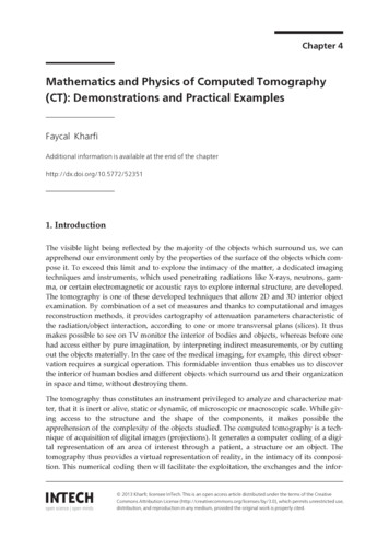
94Imaging and Radioanalytical Techniques in Interdisciplinary Research - Fundamentals and Cutting Edge ApplicationsFig. D.4. Density of the measured values in the frequency domain.For the S values of each projection in spatial domain correspond S measured values in the frequency space (measuredfor each line). Therefore, the distance ε between two consecutive values measured on a radial line in the frequencydomain (Fig. D.4) is given by:ε 2ωmax 1 SDS(D.21)A sufficient condition to obtain a good reconstruction is to ensure that the worst azimuth resolution (s) in the frequencydomain (Fig. D.4) is in the same order of radial resolution (ε). This condition can be expressed as follows:1 π1π P S2D P DS2(D.22)Thus, the ratio between the number of projections (P) and the number of rows (S) must be in the order of π / 2.An insufficient number of projections may produce a 2D or 3D reconstructed image which present many undesirableartefacts. In practice, most of the tomography detectors cannot measure below the nominal Nyquist resolutiondetermined by their dimensions or pixel size. The exploration beam is not perfectly parallel, too; this is another source oferrors on the measured data obtained especially when using a reconstruction method which assumes that the beam isparallel.In practice, insufficient number of projection generates artefacts such as those shown in figure (D.5) [3]. The projectionsof figure (D.5) have a dimension of 64x64 pixels. So the number of rows S is 64. As it has already been demonstrated, anumber P of projections around a value of 100 (P Sπ / 2) is sufficient to produce an acceptable reconstructed image.For the case of this example, it is clear that the reconstruction image obtained from 64 projections is the closest one tothe original image. The 2D reconstruction is performed using the Filtered Back-Projection method (FBP) that will bedescribed in the next section.

Mathematics and Physics of Computed Tomography (CT): Demonstrations and Practical Exampleshttp://dx.doi.org/10.5772/52351Fig. D.5. Results of 2D reconstruction of an object by FBP method of tomography and induced artifacts for differentnumber of projections: (A) original image, (B) 1 projection, (C) 3 projections, (D) 4 projections, (E) 16 projections, (F) 32projections and (G) 64 projections [7] .The number of projections is not the only parameter that affects the reconstructed image. The sampling of projections S(number of rows) and the dimensions of the grid of reconstruction will also affect the reconstructed image dramaticallyif they are not well optimizedEnd of Demonstration 41.1.2. 2D and 3D image reconstructionAs already mentioned, the inverse transformation (simple inversion) of the Fourier transformPθ(ω) can be directly used to produce the 2D reconstructed layer of μ (x, y). However, a moreefficient way and more elegant has been developed called “ Filtered Back-Projection (FBP)"making the reconstruction process less expensive and less complicated when compared to thedirect calculation of the inverse Fourier transform [1,2]. The basic idea of this method is derivedfrom the tomography principle and the scanning mode: the object (set of layers) is scannedprojection by projection from 0 to 180 which means that Pθ(t) Pθ 180(-t) and suggesting theuse of a polar coordinates rather than Cartesian square ones. As it was demonstrated thedigitization and sampling details by the right selection of P and S are very important inComputed tomography. If the projections are recorded in polar coordinates, the projectionsFourier transforms will be discrete values of a polar function. Thus, it seems appropriate towrite the 2D Fourier transform of the object function μ (x, y) in polar coordinates. The inverseFourier transform μ (x, y) of F(u, v) written in Cartesian coordinates is given by:μ(x,y) ò - ò- F(u,v).eπi(ux vy) 2dudv(13)The same inverse transform in polar coordinates is given by:μ(x,y) ò2p0 ò- F(ω,θ).eπiω(xcosθ ysinθ) 2wdwdθ(14)The substitution of x cos (θ) y sin (θ) by t and the application of Fourier Central Slice theorem,allow us to get the following expression:95

96Imaging and Radioanalytical Techniques in Interdisciplinary Research - Fundamentals and Cutting Edge Applications μ(x,y) π0 π 0 F(ω,θ).e 2πiωt ω dω dθ(15)F(ω,θ).e 2πiωt ω dω dθThe integral in brackets can be regarded as the inverse Fourier transform Pθ(t) of Pθ(ω).However, we note that it is multiplied by the function ω which plays the role of a specialramp filter function in the frequency domain. So, we define the filtered projection by: Qθ(t) - Pθ(ω) ω e 2πiωtdω(16)Thus, the object function will be simply given by:ppμ(x,y) ò éëQq (t ) ùûdθ ò éëQθ (xcosθ ysinθ) ùûdθ00(17)Knowing previously that a product (multiplication) in Fourier space (frequency domain)corresponds

ter begins with some simple, yet fundamental, concepts regarding computed tomography and the physics and mathematics at the origin of CT. As one progresses through the chapter, more detail regarding the CT technique and methodology is meet. The reader should not be alarmed if his or her part